Parallel Projections - Transformations and Projections in Computer Graphics - page 63

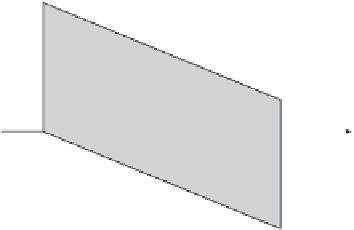
P *

θ

z

Q

P

Figure 2.13: Oblique Projections.

origin to P is the segment of size s from the origin to ( a, b, 0). The value s is therefore
the shrink factor of the oblique projection. The three quantities a , b ,and s are related
by a = s cos φ and b = s sin φ ,where φ is measured on the projection plane. The shrink
factor s is also related to the projection angle θ by tan θ =1 /s or s =cot θ .

The diagram can be drawn quite quickly because the designer used a style of drawing
called oblique projection. So long as basic rules are followed, oblique projection is
quite easy to master and it may be a suitable style for you to use in a design project.
The basic rules are outlined below.
http://www.technologystudent.com/designpro/oblique1.htm
We now consider the projecting ray from Q to ( A, B, 0). Since Q is at a distance
z from the origin, the distance on the projection plane between the origin and point
( A, B, 0) is sz . From this we obtain the relations A = sz cos φ and B = sz sin φ .The
next step is to consider the projection of a general point ( x, y, z ). All the projecting
rays are parallel, so a little thinking shows that moving a point from (0 , 0 ,z )to( x, 0 ,z )
moves its projection from ( A, B, 0) to ( x + A, B, 0). Similarly, moving a point from
(0 , 0 ,z )to(0 ,y,z ) moves its projection from ( A, B, 0) to ( A, y + B, 0). A general point
located at ( x, y, z ) is therefore projected to a point at ( x + A, y + B, 0). Thus, the rule
of oblique projections is

( x, y, z ) −→ ( x + sz cos φ, y + sz sin φ, 0) , (2.8)

whichcanbewrittenintermsofatransformationmatrix

⎛ ⎞

1 0 0

⎝ ⎠ .

P ∗ = PT =( x, y, z )

0 1 0 (2.9)

s cos φs sin φ 0

With the help of this matrix we examine the following special cases.
1. A cavalier projection. It is defined as the case where the projection angle is 45 ◦ ,
which implies s = cot(45 ◦ ) = 1. Thus, all edges and segments have shrink factors of 1.
2. A projection angle of 90 ◦ .Avalue θ =90 ◦ implies a shrink factor s = cot(90 ◦ )=
0. Matrix T of Equation (2.9) reduces to matrix T z of Equation (2.1), showing how
the oblique projection reduces in this case to an orthographic projection.