Nonlinear Projections - Transformations and Projections in Computer Graphics - page 212

A simple application of similar triangles shows that φ 0 , the latitude of tangency,
is also half the apex angle of the cone. Thus, r 0 /R =cot φ 0 . The figure also shows
that r = r 0 −

φ 0 ). It is therefore natural to
indicate the position of P ∗ on the flat projection by the polar coordinates ( r, θ ), where
r is the distance from the top (the projection of the pole) and θ is simply the sine of
the longitude of P . Table 4.63 lists the ten latitudes from 0 ◦ to 90 ◦ for R = 1 and for
φ 0 =45 ◦ (where R cot φ 0 = 1). The differences between consecutive latitudes are also
listedinthistable,anditisclearthattheyincreaseaswemoveaway(aboveorbelow)
from φ 0 .

R tan( φ − φ 0 )= R cot φ 0 − R tan( φ −

φr diff. φr diff.

0 1.999 50 0.913 0.175

10 1.700 0.300 60 0.732 0.180

20 1.466 0.234 70 0.534 0.198

30 1.268 0.198 80 0.300 0.234

40 1.087 0.180 90 0.001 0.300

Table 4.63: Ten Latitudes and Their Differences.

The most common example of this type of projection is the stereographic projection
developed by Carl Braun in 1867. It wraps the globe in a cone aligned with the rotation
axis. The cone is 1.5 times taller than the globe and is tangent to it at the 30 ◦ north
parallel. The projection center is at the south pole, not at the center of the globe, and
the resulting map is a perfect semicircle.
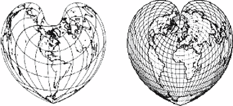
Pseudoconical projections . In this type of projection (Figure 4.64), the latitudes
are still circular arcs with a common center (concentric), and the meridians still converge
to this center but are no longer straight. Such projections have been known since the
time of Ptolemy but are not commonly used today.

Figure 4.64: Pseudoconical Projections.