Advanced Analytical Theory and Methods: Time Series Analysis - Data Science and Big Data Analytics - page 343

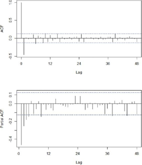
Figure 8.15 ACF of residuals from seasonal AR(1) model
Figure 8.16 PACF of residuals from seasonal AR(1) model
The ACF plot of the residuals in Figure 8.15 indicates that the autoregressive
behavior at lags 12, 24, 26, and 48 has been addressed by the seasonal AR(1) term.
The only remaining ACF value of any significance occurs at lag 1. In Figure 8.16 ,
there are several significant PACF values at lags 1, 2, 3, and 4.
Because the PACF plot in Figure 8.16 exhibits a slowly decaying PACF, and the ACF
cuts off sharply at lag 1, an MA(1) model should be considered for the nonseasonal
portion of the ARMA model on the differenced series. In other words, a (0,1,1)
× (1,0,0) 12 ARIMA model will be fitted to the original gasoline production time
series.
arima_2 <- arima (gas_prod,
order=c(0,1,1),
seasonal = list(order=c(1,0,0),period=12))
arima_2