Database Reference
In-Depth Information
8.3
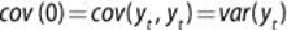
It is important to note that for , the for all
t
.
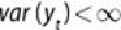
Because the , by condition (b), the variance of is a constant for all
t
. So the constant variance coupled with part (a), , for all t and some
constant , suggests that a stationary time series can look like
Figure 8.2
. In this
plot, the points appear to be centered about a fixed constant, zero, and the variance
appears to be somewhat constant over time.
Figure 8.2
A plot of a stationary series
8.2.1 Autocorrelation Function (ACF)
Although there is not an overall trend in the time series plotted in
Figure 8.2
,
it
appears that each point is somewhat dependent on the past points. The difficulty
is that the plot does not provide insight into the covariance of the variables in the
time series and its underlying structure. The plot of
autocorrelation function
(ACF)
provides this insight. For a stationary time series, the ACF is defined as
shown in
Equation 8.4
.
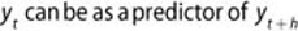
Because the cov(0) is the variance, the ACF is analogous to the correlation function
of two variables, , and the value of the ACF falls between -1 and
1. Thus, the closer the absolute value of ACF(h) is to 1, the more useful
.