Database Reference
In-Depth Information
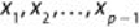
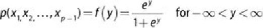
Then, based on the input variables
, the probability of an event is
shown in
Equation 6.9
.
Equation 6.8
is comparable to
Equation 6.1
used in linear regression modeling.
However, one difference is that the values of y are not directly observed. Only
the value of in terms of success or failure (typically expressed as 1 or 0,
respectively) is observed.
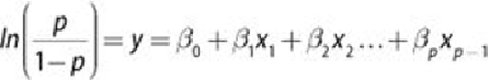
Using p to denote
,
Equation 6.9
can be rewritten in the form provided in
The quantity
, in
Equation 6.10
is known as the log odds ratio, or the
logit of p. Techniques such as Maximum Likelihood Estimation (MLE) are used
to estimate the model parameters. MLE determines the values of the model
parameters that maximize the chances of observing the given dataset. However,
the specifics of implementing MLE are beyond the scope of this topic.
The following example helps to clarify the logistic regression model. The
mechanics of using R to fit a logistic regression model are covered in the next
section on evaluating the fitted model. In this section, the discussion focuses on
interpreting the fitted model.
Customer Churn Example
A wireless telecommunications company wants to estimate the probability that
a customer will churn (switch to a different company) in the next six months.
With a reasonably accurate prediction of a person's likelihood of churning, the
sales and marketing groups can attempt to retain the customer by offering various
incentives. Data on 8,000 current and prior customers was obtained. The variables
collected for each customer follow:
•
Age
(years)