Advanced Analytical Theory and Methods: Regression - Data Science and Big Data Analytics - page 230

6.3

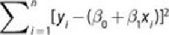
The n individual distances to be squared and then summed are illustrated in Figure
6.2 . The vertical lines represent the distance between each observed y value and
the line .

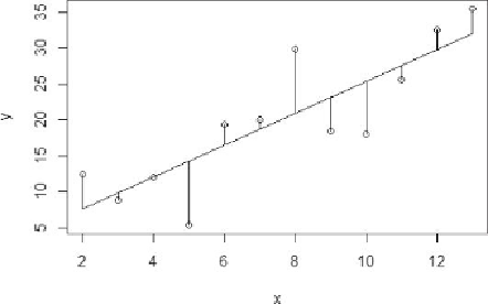
Figure 6.2 Scatterplot of y versus x with vertical distances from the observed
points to a fitted line

In Figure 3.7 of Chapter 3, “Review of Basic Data Analytic Methods Using R,” the
Anscombe's Quartet example used OLS to fit the linear regression line to each of
the four datasets. OLS for multiple input variables is a straightforward extension
of the one input variable case provided in Equation 6.3 .
The preceding discussion provided the approach to find the best linear fit to a set of
observations. However, by making some additional assumptions on the error term,
it is possible to provide further capabilities in utilizing the linear regression model.
In general, these assumptions are almost always made, so the following model,
built upon the earlier described model, is simply called the linear regression model.

Linear Regression Model (with Normally Distributed Errors)

In the previous model description, there were no assumptions made about the
error term; no additional assumptions were necessary for OLS to provide estimates
of the model parameters. However, in most linear regression analyses, it is
common to assume that the error term is a normally distributed random variable
with mean equal to zero and constant variance. Thus, the linear regression model
is expressed as shown in Equation 6.4 .