Review of Basic Data Analytic Methods Using R - Data Science and Big Data Analytics - page 146

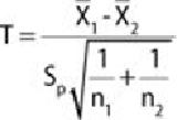
then T (the t-statistic ), given in Equation 3.1 , follows a t-distribution with
degrees of freedom (df).

Where

3.1

The shape of the t -distribution is similar to the normal distribution. In fact, as the
degrees of freedom approaches 30 or more, the t -distribution is nearly identical to
the normal distribution. Because the numerator of T is the difference of the sample
means, if the observed value of T is far enough from zero such that the probability
of observing such a value of T is unlikely, one would reject the null hypothesis that
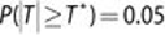
the population means are equal. Thus, for a small probability, say , is
determined such that . After the samples are collected and the
observed value of T is calculated according to Equation 3.1 , the null hypothesis (
) is rejected if .

In hypothesis testing, in general, the small probability, , is known as the
significance level of the test. The significance level of the test is the probability
of rejecting the null hypothesis, when the null hypothesis is actually TRUE . In other
words, for , if the means from the two populations are truly equal, then in
repeated random sampling, the observed magnitude of would only exceed 5%

of the time.
In the following R code example, 10 observations are randomly selected from two
normally distributed populations and assigned to the variables x and y . The two
populations have a mean of 100 and 105, respectively, and a standard deviation
equal to 5. Student's t -test is then conducted to determine if the obtained random
samples support the rejection of the null hypothesis.

# generate random observations from the two populations
x <- rnorm(10, mean=100, sd=5) # normal distribution