Database Reference
In-Depth Information
When preparing the data, one should look for signs of dirty data, as explained
in the previous section. Examining if the data is unimodal or multimodal will
give an idea of how many distinct populations with different behavior patterns
might be mixed into the overall population. Many modeling techniques assume
that the data follows a normal distribution. Therefore, it is important to know if the
available dataset can match that assumption before applying any of those modeling
techniques.
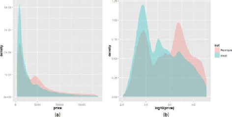
Consider a density plot of diamond prices (in USD).
Figure 3.12
(a) contains two
density plots for premium and ideal cuts of diamonds. The group of premium cuts
is shown in red, and the group of ideal cuts is shown in blue. The range of diamond
prices is wide—in this case ranging from around $300 to almost $20,000. Extreme
values are typical of monetary data such as income, customer value, tax liabilities,
and bank account sizes.
Figure 3.12
Density plots of (a) diamond prices and (b) the logarithm of
diamond prices
Figure 3.12
(
b) shows more detail of the diamond prices than
Figure 3.12
(a) by
taking the logarithm. The two humps in the premium cut represent two distinct
groups of diamond prices: One group centers around (where the
price is about $794), and the other centers around (where the
price is about $5,012). The ideal cut contains three humps, centering around 2.9,
3.3, and 3.7 respectively.
The R script to generate the plots in
Figure 3.12
is shown next. The
diamonds
dataset comes with the
ggplot2
package.
library("ggplot2")
data(diamonds)
# load the diamonds dataset from ggplot2