Biomedical Engineering Reference
In-Depth Information
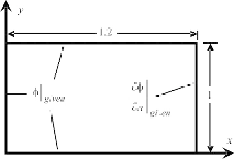
FIGURE 3.6
Schematic of the domain of interest.
procedure follows that of the “method of manufactured solution”
[22]
. Since the species
conservation (Eqn
3.1
), the energy (Eqn
3.6
), electric potential (Eqn
3.23
), and magnetic potential
(Eqn
3.30
) equations have a similar form, the same method also verifies the solution procedure for
these equations. Then, the solution of the Navier-Stokes equations (Eqns
3.3 and 3.4
) is validated
against the case of lid-driven cavity flow. The implementation of the level-set method (Eqns
3.37
and 3.38) is validated against the case of a bubble rising in a container partially filled with
aheaviermedium.
3.5.1
Verification - solution procedure of the general transient convection
diffusion equation
Figure 3.6
shows a rectangular domain in which the solution of the general transient convection-
diffusion equation (Eqn
3.42
) is sought. In the actual solution of Eqn
(3.42)
, the velocity is
known from the Navier-Stokes equations. Therefore, for verification purpose, the velocity is
assumed to be known. The velocity components are u
¼ y
and
v ¼
x. The density and diffusion
coefficients are set to
r ¼
1and
G ¼
xy, respectively. There is a source term within the rectan-
gular domain of
ae
at
x
2
y
2
S
¼
ð
þ
xy
Þ:
(3.57)
With these, it can be easily verified that the exact solution of Eqn
(3.42)
is given by
f ¼ðx
2
y
2
e
at
þ xyÞð
1
Þ:
(3.58)
For initial condition,
f ¼
0 in the whole domain. For the boundary conditions, the value of
f
is given,
except at the right boundary, i.e.,
x
1.2, where Neumann boundary condition is enforced. Solutions
were made using two different meshes, i.e., 24
¼
20 CVs with
D
t
¼
0.010 s and 48
40 CVs with
D
0.010 s is
sufficient to achieve mesh-independent solution. The predicted solutions agree very well with the exact
solution of Eqn
(3.58)
.
t
¼
0.005 s. These solutions are shown in
Fig. 3.7
. A mesh of 24
20 CVs with
D
t
¼


Search WWH ::

Custom Search