Characterization techniques - Micromixers Fundamentals Design and Fabrication - page 308

The parabolic estimator assumes a parabolic fitting function for the correlation peak:

Ax 2

f ð x Þ¼ þ Bx þ C : (8.19)

In this case, the refined position of the peak is

R ð x 1 ; y Þ R ð x þ 1 ; y Þ

x 0 ¼ x þ

Þ ; 2 R ð x 1 ; y Þ 4 R ð x ; y Þþ 2 R ð x þ 1 ; y

(8.20)

R ð x ; y 1 Þ R ð x ; y þ 1 Þ

y 0 ¼ y þ

Þ : 2 Rðy; x 1 Þ 4 Rðx; yÞþ 2 Rðx; y þ 1

The Gaussian estimator assumes a Gaussian distribution of the correlation peak:

C exp "

#

2

ð x 0 x Þ

f ð x Þ¼ : (8.21)

k

The position of the peak can the be estimated as

ln R ð x 1 ; y Þ ln R ð x þ 1 ; y Þ

x 0 ¼ x þ

Þ ; 2ln R ð x 1 ; y Þ 4ln R ð x ; y Þþ 2ln R ð x þ 1 ; y

(8.22)

ln R ð x ; y 1 Þ ln R ð x ; y þ 1 Þ

y 0 ¼ y þ

Þ : 2ln R ð x ; y 1 Þ 4ln R ð x ; y Þþ 2ln R ð x ; y þ 1

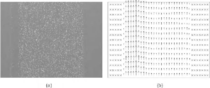
Figure. 8.10 shows a typical particle image and the corresponding evaluated velocity field
(micro-PIV).
The results of micro-PIV can be improved by several techniques, such as removing the background,
improving the particle density, and reducing the noise in the correlation matrix.

FIGURE 8.10

Typical results of a micro-PIV measurement: (a) particle image (single frame, double exposure) and (b) evaluated
velocity field.