Cryptography Reference
In-Depth Information
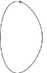
> display(el, pts, txt, labels = [" ", " "], scaling = constrained);
Next we are going to add
P
to itself. For this we have to compute the tangent to
the curve at
P
. Using the formula for the tangent we compute the partial derivatives
of the polynomial
F
, evaluate them at
P
and we obtain
3
:
> T := (eval(diff(F, x), [x=-1, y=2]))*(x+1)+(eval(diff(F, y), [x=-1, y=2]))*(y-2);
x-7+4y
An alternative way of computing the tangent is to write it in the form
y
=
m
(
x
+
1
. This slope may
be computed by using implicit differentiation on
F
with respect to
x
and evaluating
the result at
P
and we use Maple to do so and to obtain the equation of the tangent
(if the tangent line were vertical, which is not the case here, then the slope would not
be defined and Maple would give a “division by zero error” that we could interpret
as meaning that
m
)
+
2 where
m
is the slope of the curve at the point
P
=
(
−
1
,
2
)
=∞
):
> y = (eval(implicitdiff(F, y, x), [x = -1, y = 2]))*(x+1)+2;
y = - x/4 + 7/4
Of course, this equation defines the same line. Next we compute the third point
of intersection of this line with the curve:
3
It is also possible to write the result as an equation with the polynomial equated to 0 but this is
not necessary to plot the curve because Maple knows what to do when asked to plot a polynomial.