Steganography in Halftone Images - Visual Cryptography and Secret Image Sharing - page 363

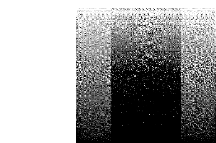
FIGURE 13.18
Image Y obtained by overlaying Y 1 in Figure 13.16 and Y 2 in Figure 13.17.

the corresponding row in X in Figure 13.19. Three such curves are obtained
with 3 values of T, namely T = 5; 10; 15. Also shown in the gure is the
theoretical behavior as predicted by (13.35). It can be observed from the
figure that as T increases, the average intensity curves appear to converge to
the theoretical curve, as expected.
We also compute the difference between the average intensity in the W b
and the W w regions for each row of Y , and plot this intensity against the
average intensity of the corresponding row in X in Figure 13.20. Similarly,
the contrast is computed and plotted in Figure 13.21. Also shown in the two
figures are the theoretical behavior predicted by (13.36) and (13.37). It can be
observed that as T increases, the intensity curves and the contrast curves
appear to converge to the corresponding theoretical curves, as expected.
Next, we analyze DHSED and make a comparison with DHCED. Since
DHSED forces Y 1 and Y 2 to be identical in W w , both y 1 (i;j) and y 2 (i;j) are
identical in the left half of R and the probability distribution is

P[y(i;j) = 255] = P[y 1 (i;j) \y 2 (i;j) = 255] = P[y 1 (i;j) = 255] = A=255
(13.38)
such that E[y(i;j)] = A. For any (i;j) in W b , the corresponding pixel values
in Y 1 and in Y 2 are error diffused with relative random phase. Thus, the local
intensity for Y 1 and Y 2 is

E[y 2 (i;j)] = E[y 1 (i;j)] = A (13.39)