Biomedical Engineering Reference
In-Depth Information
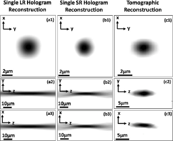
Fig. 4.12
(
a1
-
a3
) show the reconstructed images of a 2m diameter microsphere in x-y, y-z, and
x-z planes, respectively, using a single LR hologram. (
b1
-
b3
) show the reconstructed images of a
2m diameter microsphere in x-y, y-z, and x-z planes, respectively, using a SR hologram. (
c1
-
c3
)
show the computed tomograms in the x-y, y-z, and x-z planes for the same microparticle, obtained
by using the field-portable lensless tomographic microscope shown in Fig.
4.13
Since we correct for the diffraction between the object and the sensor (i.e.,
hologram plane) by digital holographic reconstruction algorithms as discussed in
earlier sections, the use of a back-projection algorithm, as opposed to a diffraction
tomography approach, only ignores the diffraction within the object. This approx-
imation can be justified by the modest NA (0.3-0.4) and the relatively long DOF
of our lensfree projection images. We can denote the sample's 3D transmission
function as s.x
;y
;
z
/,where.x
;y
;
z
/ defines a coordinate system whose
z-axis is aligned with the illumination angle () at a particular projection. Ignoring
multiple scattering within the sample and by assuming that it weakly scatters the
incident light [
60
], after phase recovery (or twin-image elimination) steps, each
amplitude projection image yields the 2D line integral of our 3D object function,
that is,
R
<DOF>
j
s.x
;y
;
z
/
j
d
z
. That is, a projection image along a given angle
can be approximated to represent a rectilinear summation of the amplitudes of
the transmission coefficients of the 3D object over a length scale of one depth of
focus (DOF) around z
0
,wherez
0
is the depth for which the tomogram is to be