Environmental Engineering Reference
In-Depth Information
Total
Uplifting
1.0
Piping
0.8
Sliding
Overturning
0.6
Reinforcement failure
0.4
Shear failure
0.2
Piping toe
0.0
Crest level
0.0
2.0
4.0
6.0
8.0
10.0
Indication extreme
water level
Water level (m OD)
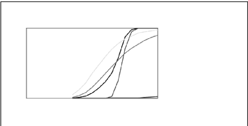
Fig. 15.6
A typical fragility curve based on the reliability analysis for a defence in the Thames Estuary. (See the colour
version of the figure in Colour Plate section.)
the failure probabilities are conditional on the
loads) and the probability of failure is assessed for
specific loading events (by integrating the proba-
bility distributions assigned to variables and para-
meters that describe the strengths (S) of the asset
over the failure region, i.e. the load exceeds the
sampled strength).
A set of high-level fragility curves that repre-
sent the typical assets found in the UK provide a
common reference of asset fragility. These high-
level curves are based upon a limited number of
readily available asset characteristics (e.g. from
the NFCDD). The high-level classification (as de-
fined by the RASP (Risk Assessment for Strategic
Planning) defence types; Hall et al. 2003) differ-
entiates the assets first by seven major types (flu-
vial - not exposed to wave action; or coastal -
exposed to wave action; vertical or sloping) and
then by their width (narrow,
<
6-m crest; or wide,
>
6-m crest) and the nature and extent of the
surface cover protection. A seventh classification
of high ground is also included. A restricted set of
limit state equations are then used within a reli-
ability analysis to develop the fragility curves for
eachRASP defence based on three indicator failure
modes:
1 Overtopping - periodic overflow of the defence
due to wave action (coastal defences only).
2 Overflow - when the water level is above the
defence (coastal and fluvial).
3 Piping - when the water level is below the crest
level of the defence (fluvial only) (Environment
Agency 2007a).
To determine an initial estimate of the fragility
of a specific asset, the high-level fragility curves
can be combined with local-scale data on asset
condition (either measured or estimated), crest
level of the asset, as well as the local loading
conditions to which the asset is exposed. This
allows the high-level fragility curves to utilize
available local data (without increasing analysis
effort). [Note: For example, Gouldby et al. (2010)
provide a full list of the local parameters used to
complement the high-level fragility curves as part
of the National Flood Risk Assessment routinely
undertaken for England and Wales.]
In many cases it is appropriate to refine the
understanding of asset reliability beyond the
high-level fragility curves described above. This
may be in response to the importance of a partic-
ular asset in terms of managing risk (e.g. a major
structure such as the Thames Barrier) or where
doubt remains as howbest to intervene and further
investigation is required. A structured procedure
to derive more credible asset-specific fragility
curves is provided in Table 15.2.