Environmental Engineering Reference
In-Depth Information
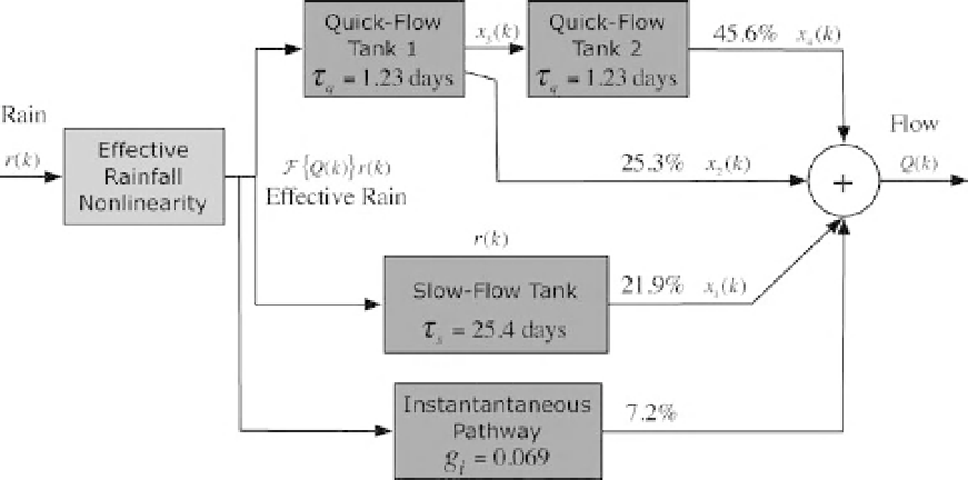
Fig. 9.9
The Data-Based Mechanistic (DBM) model of the Leaf River: here,
t
q
and
t
S
are the quick and slow residence
times, while the percentage figures denote the percentage of flowpassing down the indicated pathways. (See the colour
version of this Figure in Colour Plate section.)
eigenvalues may be superior in statistical terms. A
fourth-order model with three quick-flow tanks was
rejected because of clear identifiability problems.
The identified third-order, constrained DBM
model was estimated from an estimation dataset
of 366 days over 1952-1953 and is shown diagram-
matically in Figure 9.9, where the output flow is
now denoted by Q
k
, rather than the more general
output variable y
k
used in previous sections, in
order to aid comparison with the HYMOD dia-
gram in Figure 9.8: both have an input 'effective
rainfall' nonlinearity, although these are not of the
same form; and both have a 'parallel pathway' flow
structure consisting of 'quick' and 'slow' flow
tanks, although HYMOD has the additional
quick-flow tank, mentioned above, which is ef-
fectively replaced in the DBM model by the
'instantaneous' pathway, represented by a simple
gain coefficient with no dynamics.
Themain difference between themodels is that
whereas in HYMOD the a priori conceptualized
structure is fitted to the data in a hypothetico-
deductive manner, the DBM model structure is
identified statistically from the data in an induc-
tive manner, without prior assumptions other
than that the data can be described by a nonlinear
differential equation or, as in this case, an equiv-
alent discrete-time difference equation: see, for
example, the discussion in Young (2002). It is
necessary to stress again that the DBMmodel here
is constrained to some extent in order tomatch the
structure of the HYMOD model and this would
not normally be the case in DBM modelling (see
discussion under 'Comments' below).
The DBM model is estimated initially in a
nonlinear Transfer Function (TF) form since it is
possible to do this by exploiting easily available,
general TF estimation tools, such as those in the
CAPTAIN Toolbox mentioned previously. This
contrasts with direct estimation of a specified
model in state space model form, where a custom-
ized algorithm is required. Moreover, it can be
shown that there are statistical advantages in
estimating the minimally parameterized transfer
function model and it can be transformed easily
into any selected state space model form that has
relevance to the problemat hand: for example, one
that has a useful physical significance. The DBM
model in Figure 9.9 is obtained in this manner and
it relates to the following state space form, which