Information Technology Reference
In-Depth Information
emerge therewith [7]. Leaving details, the boundary condition must lead to a well-posed
problem, as well as be adequate to the phenomenon being modelled from the physical
standpoint. To overcome this difficulty, we suggest it should be used the map swap —
instead of
λ
k
being varied from the zero meridian around the sphere and
ϕ
l
from the
South pole to the North, one should change the coordinate map from (10) to
.
(11)
(
λ
k
,ϕ
l
):
λ
k
∈
Δλ
2
,ϕ
l
∈
S
(2)
Δλ
2
π
2
+
Δϕ
2
,
3
π
Δϕ
2
Δλ,Δϕ
=
,π−
−
2
+
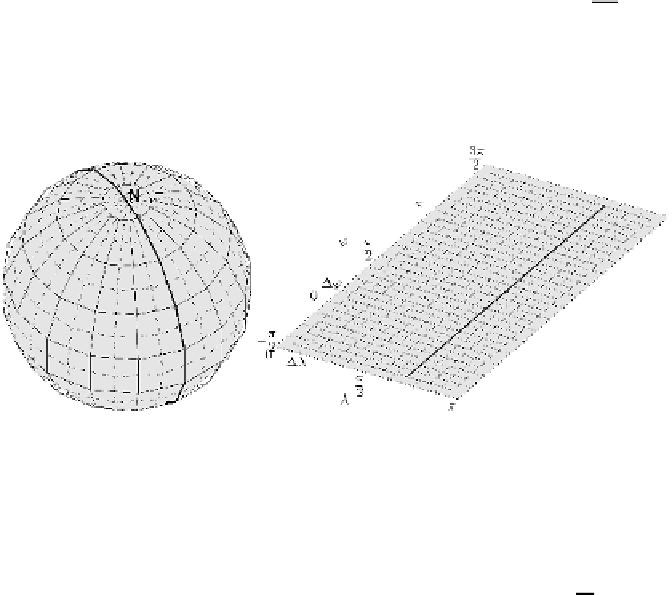
Obviously, both maps cover the entire sphere and consist of the same grid nodes. The
use of map (11) allows treating the solution as periodic while computing in
ϕ
, similarly
to how it is in
λ
(Fig. 2).
Fig. 2.
The grid shown in the solid line is used while solving in
ϕ
. This allows considering the
sphere as a periodic domain in the latitude, without the necessity of constructing boundary con-
ditions at the poles.
Having armed ourselves with (10)-(11), now we are ready for the discretisation of
the split 1D problems.
Typically, let
G
kl
=
G
(
λ
k
,ϕ
l
)
,where
G
is any of the functions
T,D,f
. Approxi-
mate (8)-(9) as follows
D
k
+1
/
2
T
n
+
2
k
− T
k
1
R
2
cos
2
ϕ
1
Δλ
T
k
+1
− T
k
Δλ
T
k
− T
k−
1
Δλ
=
− D
k−
1
/
2
τ
A
Δλ
T
k
f
n
+
2
k
+
,
(12)
2
D
l
+1
/
2
− T
n
+
2
l
T
n
+1
l
1
R
2
|
cos
ϕ
l
|
1
Δϕ
T
l
+1
− T
l
Δϕ
T
l
− T
l−
1
Δϕ
=
− D
l−
1
/
2
τ
A
Δϕ
T
l
f
n
+
2
l
+
,
(13)
2


Search WWH ::

Custom Search