Information Technology Reference
In-Depth Information
where
α
,
D
=
μ
(
T
n
)
(7)
while
T
n
=
T
(
λ, ϕ, t
n
)
. Then we split equation (6) by coordinates as follows [4]
D
R
cos
ϕ
∂T
∂t
=
A
λ
T
+
f
2
≡
1
R
cos
ϕ
∂
∂λ
∂T
∂λ
f
2
+
,
(8)
D
cos
ϕ
R
∂T
∂t
=
A
ϕ
T
+
f
2
≡
1
R
cos
ϕ
∂
∂ϕ
∂T
∂ϕ
f
2
+
.
(9)
This means that in order to find the solution at a time moment
t
n
+1
one has first to solve
equation (8) in
λ
using the function
T
(
λ, ϕ, t
)
at
t
n
as the initial condition. Then, taking
the resulting solution as the initial condition, one has to solve (9) in
ϕ
. The outcome
will be the (approximate) solution to (1) at
t
n
+1
. In the next time interval
(
t
n
+1
,t
n
+2
)
the succession has to be repeated, and so on.
Two challenges are met here.
First, because the term
R
cos
ϕ
vanishes at
ϕ
=
±π/
2
, equations (8)-(9) have no
sense at the poles. Therefore, defining the grid steps
Δλ
=
λ
k
+1
− λ
k
and
Δϕ
=
ϕ
l
+1
− ϕ
l
, we create a half-step-shifted
λ
-grid
.
(10)
(
λ
k
,ϕ
l
):
λ
k
∈
Δλ
2
,ϕ
l
∈
S
(1)
Δϕ
2
Δϕ
2
Δλ
2
π
,
π
Δλ,Δϕ
=
,
2
π
+
−
2
+
2
−
The half step shift in
ϕ
allows excluding the pole singularities, and therefore the cor-
responding finite difference equation will have sense everywhere on
S
(1)
Δλ,Δϕ
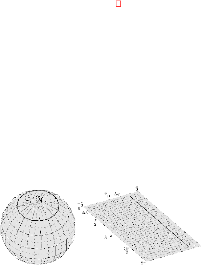
(Fig. 1).
The equation is enclosed with the periodic boundary condition, since the sphere is a
periodic domain in
λ
.
Fig. 1.
The grid shown in the solid line is used while solving in
λ
. The semi-integer shift in
ϕ
allows excluding the pole singularities, which keeps the equation to have sense on the entire
sphere.
Second, while solving in
ϕ
, equation (9) has to be enclosed with two boundary con-
ditions at the poles. It is well known, however, that the construction of an appropriate
boundary condition is always a serious problem, because a lot of undesired effects may


Search WWH ::

Custom Search