Graphics Reference
In-Depth Information
Since the gradient at a pixel indicates the direction of greatest change, we can
locally compute the isophote direction as the unit vector perpendicular to the
gradient; that is,
unit
I
(
x
,
y
)
−
I
(
x
,
y
+
1
)
∇
⊥
I
(
x
,
y
)
=
(3.29)
I
(
x
+
1,
y
)
−
I
(
x
,
y
)
Putting all this together mathematically, the pixel intensities that fill the hole
should satisfy the partial differential equation (PDE):
2
I
)
·∇
⊥
I
∇
(
∇
=
0
(3.30)
2
I
That is, the change in the Laplacian
∇
(
∇
)
should be zero in the direction of
∇
⊥
I
. Ideally, we could solve Equation (
3.30
) by creating an image that
changes as a function of time according to the following PDE:
the isophote
∂
I
2
I
)
·∇
⊥
I
=∇
(
∇
(3.31)
∂
t
When the image stops changing,
∂
I
∂
0 and thus the solution satisfies Equation (
3.30
).
In practice, we approximate Equation (
3.31
) with discrete time steps, letting
t
=
I
n
+
1
(
x
,
y
)
=
I
n
(
x
,
y
)
+
(
∇
t
)
U
n
(
x
,
y
)
,
∀
(
x
,
y
)
∈
(3.32)
is derived from a discrete approximation of
Equation (
3.30
), with the usual approximations of the gradient and the Laplacian.
Bertalmio et al. recommended several enhancements to the implementation, includ-
ing interleaved steps of
anisotropic diffusion
to smooth the intermediate images
without losing edge definition. A typical result of inpainting an image with thin holes
is illustrated in Figure
3.18
, showing several steps of evolution.
Note that we could achieve a similar result using the Poisson compositing tech-
nique fromtheprevious section, simplyby setting the guidance vector field
The update image
U
n
(
x
,
y
)
(
S
x
,
S
y
)
=
0
(a)
(b)
(c)
(d)
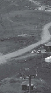
Figure 3.18.
(a) The original image. (b) The inpainting mask. (c) After 4,000 iterations of PDE-
based inpainting, the wire locations are still perceptible as blurry regions. (d) After 10,000
iterations of PDE-based inpainting, the wires have disappeared.