Graphics Reference
In-Depth Information
X
j
f(
X
) = 0
f(
X
) = 1
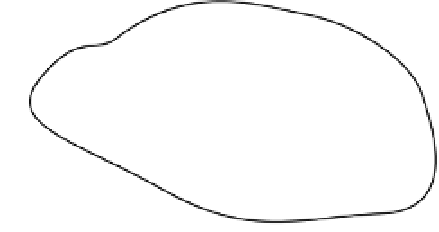
Figure 8.39.
The setup for Poisson surface reconstruction. 3D sample points (black dots) are
viewed as locations where the gradient is large and points inward.
=
X
i
X
j
2
. Now we can compute
f
where
r
ij
at any 3D location we like, and
apply the same marching-cubes technique to obtain the isosurface. This approach
3D to surface interpolation was proposed by Turk and O'Brien [
502
], though it can be
traced back to the thin-plate spline techniques of Bookstein [
53
] and earlier.
However, for scans with more than a few thousand data points, forming and solv-
ing the linear systeminEquation (
8.23
) quickly becomes computationally intractable.
Carr el al. [
82
] showed how such techniques could be made feasible using fast mul-
tipole methods, which use near-field and far-field approximations to compute the
radial basis functions efficiently. Such approaches also allow the specification of a
desired fitting accuracy, which is useful for merging multiple LiDAR scans that may
not overlap exactly after registration. They showed howmerged LiDAR datasets con-
taining hundreds of thousands of points could bewell approximatedwith a triangular
mesh in a matter of minutes.
On the other hand, radial basis function approaches may smooth over sharp fea-
tures in the data that we want to preserve, introduce pieces of surface far from the
original data points, and perform badly in the presence of outliers or poorly sampled
data. More recent approaches to surface reconstruction (e.g.,[
353
,
245
]) address these
problems.
Finally, we mention one of the most effective 3D data fusion techniques,
Poisson
surface reconstruction
, proposed by Kazhdan et al. [
232
]. Like the previous tech-
niques, we compute a function
f
−
(
X
)
3
; however, this function has a very
different interpretation, as sketched in Figure
8.39
. We define
f
(
X
)
defined on
R
(
X
)
=
0 for points
outside the surface to be reconstructed, and
f
1 for points inside the surface to
be reconstructed. Therefore, the gradient of the function is identically zero, except
for points
X
on the surface, at which the gradient is very large (theoretically infinite).
The observed range data points
(
X
)
=
are viewed as samples where the gra-
dient is known; that is, its norm is large and it points inward along the estimated
normal.
This problem, in which we have samples of the gradient of a function at
several points and want to reconstruct the function everywhere, naturally lends
itself to Poisson reconstruction techniques, as we described for image editing in
Section
3.2
. The approach proposed by Kazhdan et al. has several advantages: it's
relatively robust to sparse or noisy gradient samples, it generates surfaces that stick
closely to the original data without requiring normal constraints, and it allows the
use of a multiresolution (octree) data structure to represent the result instead of
{
X
j
,
j
=
1,
...
,
n
}


