Graphics Reference
In-Depth Information
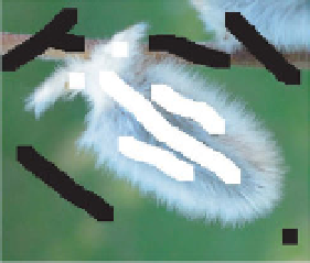
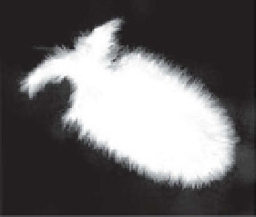
(a)
(b)
(c)
Figure 2.13.
(a) An image with (b) foreground and background scribbles. (c) The
α
matte com-
puted using closed-form matting, showing that good estimates are produced in fine detail
regions.
Choosing the right window size for closed-form matting can be a tricky problem
depending on the resolution of the image and the fuzziness of the foreground object
(which may not be the same in all parts of the image). He et al. [
192
] considered
this issue, and showed how the linear system in Equation (
2.41
) could be efficiently
solved by using relatively large windows whose sizes depend on the local width of the
uncertain region
in the trimap. The advantage of using large windows is that many
distant pixels are related to each other, and the iterative methods typically used to
solve large systems like Equation (
2.41
) converge more quickly.
U
2.4.4
Recovering
F
and
B
from
α
After solving the linear system in Equation (
2.41
) we obtain
α
values but not estimates
of
F
and
B
. One way to get these estimates is to treat
and
I
as constant in thematting
equation and solve it for
F
and
B
. Since this problem is still underconstrained, Levin
et al. suggested incorporating the expectation that
F
and
B
vary smoothly (i.e., have
small derivatives), especially in places where thematte has edges. The corresponding
problem is:
α
N
2
1
I
i
−
(α
i
F
i
+
(
−
α
i
)
B
i
)
min
F
i
,
B
i
1
(2.42)
i
=
2
2
2
2
+|∇
α
|
∇
x
F
i
+∇
x
B
i
+|∇
α
|
∇
y
F
i
+∇
y
B
i
x
i
y
i
where the notation
∇
x
I
represents the gradient of image
I
in the
x
direction,
which is a scalar for a grayscale image and a 3-vector for a color image. Solving
Equation (
2.42
) results in a sparse linear system instead of a problem solved indepen-
dently at every pixel, since the gradients force interdependence between the pixels
(see Problem
2.18
).
2.4.5
The Matting Laplacian's Eigenvectors
Levin et al. observed that even before the user imposes any scribbles on the image to
be matted, the eigenvectors of the matting Laplacian corresponding to the smallest
eigenvalues reveal a surprising amount of information about potentially good mat-
tes. For example, Figure
2.14
illustrates the eight eigenvectors corresponding to the