Graphics Reference
In-Depth Information
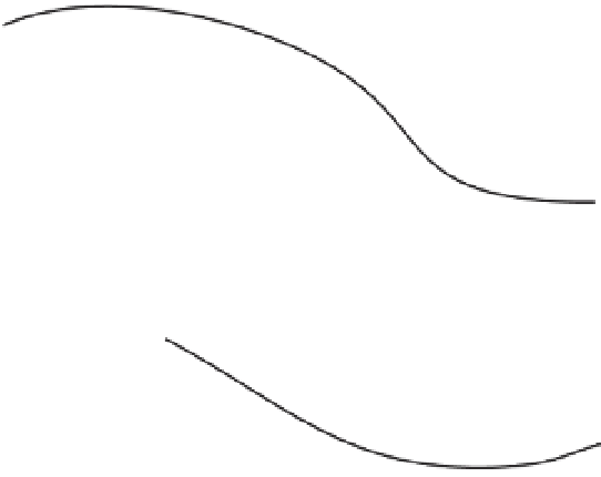
Motion 1
w = 0
w = 0.25
w = 0.5
Motion 2
w = 0.75
w = 1
Figure 7.15.
Interpolating the root position and orientation for a transition between two
motions, for different values of the weight
w
. In this case, the intermediate positions are cre-
ated with linear interpolation and the intermediate orientations are created with spherical linear
interpolation.
a curved line given by linearly interpolating between the starting and ending velocity
vectors [
396
]). Figure
7.15
illustrates the idea.
The interpolated motion created by this process is aligned to the time indices of
the first motion; we can speed up or slow down the motion in the transition region
as desired. A natural choice is to remap the interpolated motion to have duration
1
2
T
)
(
+
.
Figure
7.16
illustrates an example of a motion blend using this technique, transi-
tioning froma normal walkingmotion to a sneakingmotion. The result is perceptibly
worse without dynamic time warping. For example, in the third frame of Figure
7.16
c,
both feet are well off the ground, and in the fourth frame the figure is leaning for-
ward on both toes. The figure seems to stutter and glide across the ground, and never
makes a satisfactory transition to the crouching posture.
Kovar and Gleicher [
252
] extended this approach by enforcing that the dynamic
time warping path doesn't take too many consecutive horizontal or vertical steps
(i.e., mapping the same frame from one sequence onto many frames of the other).
They then fit a smooth, strictly increasing spline to the dynamic time warping path,
which they called a registration curve. They also generalized the approach to allow
the blending of more than two motion sequences. Instead of applying dynamic time
warping, Rose et al. [
395
] modeled the correspondence as a piecewise-linear path
defined by annotated keyframe correspondences (e.g., matching points in a walk
cycle).
The monotonic function defining the weights
w
i
could be a simple linear transi-
tion, or a function with non-constant slope, e.g., arising from radial basis functions
[
395
], B-splines [
266
], or the desire for differentiability [
254
]. In general, whenwewant
to blend between more than two motions, any of the scattered data interpolation
techniques from Section
5.2
can be applied.
T