Graphics Reference
In-Depth Information
general form
g
i
(
θ
(
t
))
≤
b
i
(7.28)
Problems withnonlinear constraints are generallymuch harder to solve than those
with linear constraints, especially at interactive rates. An alternative is to include the
constraints as weighted penalty terms in an unconstrained cost function, e.g., by
adding cost function terms of the form
C
constraint
(
θ
(
t
))
=
max
(
0,
g
i
(
θ
(
t
))
−
b
i
)
(7.29)
As with Equation (
7.23
), the result of minimizing a sum of weighted cost func-
tion terms is not guaranteed to strictly satisfy any of the constraints given in each
term. That is, the marker positions will generally not agree exactly with the forward
kinematics model, and the desired range of motion constraints may not be exactly
satisfied. Tolani et al. [
491
] proposed to mitigate this problem using a hybrid analyti-
cal/numerical approach that was able to solve for most of the degrees of freedom of
a simplified kinematic chain in closed form.
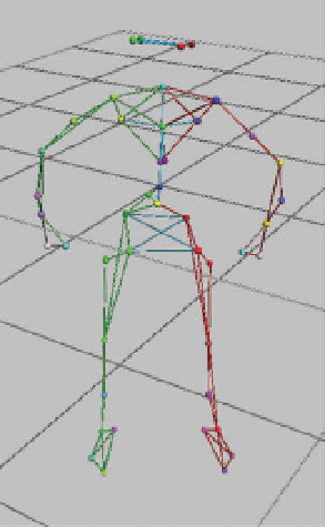
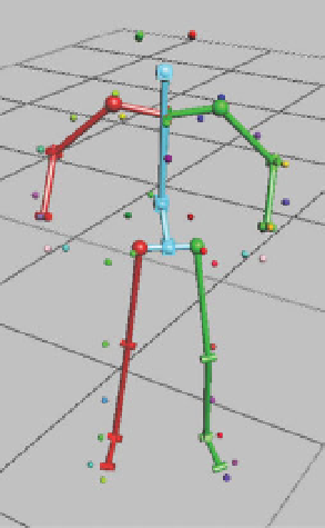
Figure
7.11
illustrates an example result of optimization-based inverse kinematics,
rendering rawmotion capturemarkers alongside the estimated skeletal pose fromthe
same perspective.
In addition to simple, uncoupled limits on the range of motion of each joint that
are independent at each point in time, we can incorporate dependencies on joint
limits, as discussed by Herda et al. [
195
]. For example, the range of motion of the
knee joint varies depending on the position and orientation of the hip joint. Such
dependencies can be characterized by analyzing motion capture training data to
(a)
(b)
Figure 7.11.
An example inverse kinematics result. (a) The original motion capture markers,
which form the constraints for an optimization-based inverse kinematics problem. Lines are
drawn between markers on the same body part to give a sense of the pose. (b) The estimated
skeletal pose from the same perspective. We can see that the markers are sometimes quite far
from the skeleton.