Graphics Reference
In-Depth Information
it. The
Levenberg-Marquardt
algorithmcommonly used for bundle adjustment uses
the approximation
2
F
∂
θ
∂
t
t
)
J
t
t
I
2
(
θ
)
≈
J
(
θ
(
θ
)
+
λ
(6.66)
t
is a tuning parameter that varies with each iteration and
I
is an appropri-
ately sized identity matrix. The reasoning behind this approximation is described in
Appendix
A.4
.
Therefore, at eachLevenberg-Marquardt iterationcorresponding toEquation (
6.63
),
we must solve a linear system of the form
where
λ
t
)
J
t
t
I
t
J
(
θ
t
t
(
J
(
θ
(
θ
)
+
λ
)δ
=
)(
x
−
f
(
θ
))
(6.67)
t
t
t
+
1
. These are also known as the
where
δ
is the increment we add to
θ
to obtain
θ
normal equations
for the problem.
If we treated Equation (
6.67
) as a generic linear system, we would waste a lot
of computation since the Jacobian matrix
J
has many zero elements. That is, each
reprojection
ˆ
x
j
only depends on one camera matrix and one scene point, so all of
the derivatives
∂
f
j
k
that don't involve the corresponding camera or
point. Thus, while there may be hundreds of camera parameters, thousands of scene
points, and tens of thousands of feature matches in a realistic bundle adjustment
problem, the matrix
J
is very
sparse
. The matrix
J
J
in Equation (
6.67
) will also be
sparse (but less so). Figure
6.14
illustrates the structure of
J
and
J
J
for a simple
problem, to illustrate the sparsity pattern.
We can exploit this sparsity pattern tomore efficiently solve Equation (
6.67
). From
Figure
6.14
b, we can see that Equation (
6.67
) can be written in terms of submatrices
∂
θ
k
will be zero for
θ
P
1
P
2
P
3
X
1
X
2
X
3
X
4
x
11
x
12
x
13
x
14
x
21
x
22
x
23
x
24
x
31
x
32
x
33
x
34
P
1
P
2
P
3
X
1
X
2
X
3
X
4
P
1
P
2
P
3
X
1
X
2
X
3
X
4
(a)
(b)
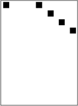
Figure 6.14.
Suppose we have a bundle adjustment problem in which three cameras observe
four points. (a) The structure of the Jacobian
J
is indicated by dark blocks for nonzero elements
and white (empty) blocks for zero elements. The rows index feature observations while the
columns index camera and scene parameters. (b) The structure of
J
J
for the same problem.
Both matrices are even sparser when all the features aren't seen by all the cameras (which is
typical in a real matchmoving problem, see Figure
6.16
).