Agriculture Reference
In-Depth Information
1000
3 Dominant,
3 Dominant,
3 additive
3 Dominant,
3 additive
3 additive
800
All additive
All additive
5 Dominant,
5 Dominant,
1 additive
5 Dominant,
1 additive
1 additive
600
1 Dominant,
1 Dominant,
5 additive
1 Dominant,
5 additive
5 additive
400
200
0
500
510
520
530
540
550
560
Yield
570
580
590
600
610
620
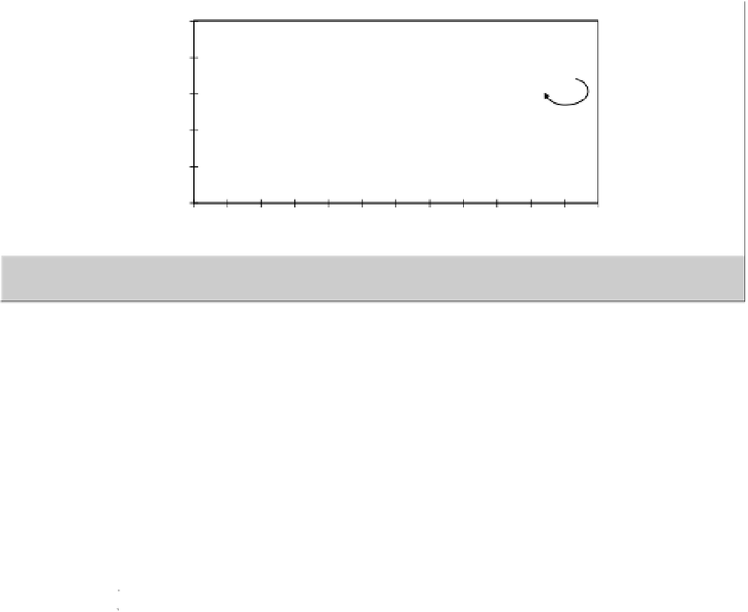
Figure 5.3
The degree of skewness of a six loci two-allele system is shown for no dominance, one dominant locus, three
dominant loci and five dominant loci. Note that increasing the number of dominant loci results in greater skewness.
of the F
, of recombinant inbred lines would be
equal to the mid-parental value, the same as if no
dominance (or indeed linkage) existed. Therefore, if
dominant effects are adversely effecting selection in
plant breeding, then increased rounds of selfing can
eliminate these effects.
can be either
positive or negative (i.e. the F
1
has higher or lower
performance than
m
, respectively).
Using these three parameters we can now proceed to
determine the expected performance of any generation.
We have:
Unlike
[
a
]
which is always positive,
[
d
]
∞
High parent ( P
1
)
=
Consider again the inheritance model that we have for
additive effects:
m
+
a
;
Low parent ( P
2
)
=
−
m
a
;
−
−
−
F
1
=
+
m
d
P
2
F
1
P
1
500
560
m
620
Assume that the P
1
, P
2
and F
1
generations are grown so
that
m
,
can be calculated from their means,
then it can thus be seen why
m
,
a
and
d
are referred to
as the
components of the generation means.
[
a
]
and
[
d
]
[
a
]
[
a
]
As we have seen the F
1
performance does not always
coincide with the mid-parent value. In the two loci case
we had:
−
−
−
P
2
F
1
P
1
m
−
[
a
]
m
+
[
a
]
m
+
[
a
]
−
−
−
P
2
F
1
P
1
m
500
560
580
620
[
a
]
[
a
]
m
[
d
]
P
1
,
P
2
and
F
1
three further generations
In addition to
So we now need to add a second parameter to the
model
are commonly considered:
[
]
d
which represents the amount of dominance,
and where:
•
The F
2
generation (i.e. F
1
selfed)
]=
F
1
−
[
d
m
The
back-cross generation
F
1
×
•
P
1,
which is termed the
B
1
generation
and from this we have:
F
1
=
The
back-cross generation
F
1
×
•
P
2
, which is termed
m
+[
d
]
the B
2
generation