Random Variable - Random Signals and Processes Primer with MATLAB - page 62

a b

x

F x ( )

1

x )

x

F x (

F x ( |X ≤ 1)

x

1 23 4

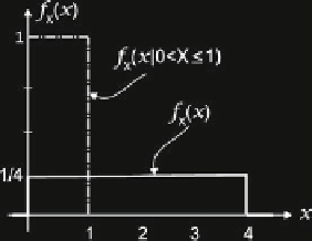
Fig. 2.27 Conditional PDF and distribution from Example 2.5.2. ( a ) Densities. ( b ) Distributions

2.6 Transformation of a Random Variable

2.6.1 Introduction

Random signals often pass through devices which transform their characteristics.
A typical example of this is noise in telecommunications systems. The problem
arises when trying finding the characteristics of the random variable after its
transformation, if the characteristics of the random variable before transformation
are known. In denoting random variables before and after transformation (as X and
Y , respectively), we have:

Y ¼ gðXÞ; (2.131)

where g denotes the functional relation between X and Y (Fig. 2.28 ). The same
relation holds for the corresponding ranges

y ¼ gðxÞ: (2.132)

The result depends on the type of the transformation. Here, we consider a unique
transformation in which the same input value always corresponds to the same
output value. The unique transformation can be a monotone and a nonmonotone .
In a monotone transformation there is only one output value for each input value, as
shown in Fig. 2.29a . However, in a nonmonotone transformation, two or more input
values correspond to only one output value, as illustrated in Fig. 2.29b .

2.6.2 Monotone Transformation

Consider the monotone transformation of the input random variable X , Y ¼ g ( X ).
If the input random variable X is in the interval