Normal Random Variable - Random Signals and Processes Primer with MATLAB - page 284

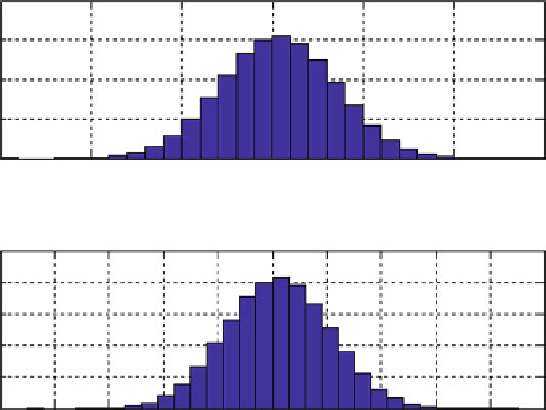
Input random variable X

0.8

0.6

0.4

0.2

0
- 2

- 1 0 1 2 3 4

cells

Output random variable Y

0.2

0.15

0.1

0.05

0

- 4 - 2 0 2 4 6

cells

8 10 12 14 16

Fig. 4.38 Input and output estimated PDFs

Solution The random variables X 1 and X 2 and their sum are shown in Fig. 4.39 .
Observing the random variable Y , we can easily conclude that the variable Y is also
a normal random variable. This is confirmed by estimating the PDFs of the
variables, X 1 , X 2 , and Y (shown in Fig. 4.40 ).
Exercise M.4.8 (MATLAB file: exercise_M_4_8.m ) Show the CLT considering
the sum of five uniform random variables in the interval [1, 4].

Solution We generate a uniform random variable and present the sum of 2, 3, 4, and
5, uniform variables in Fig. 4.41 , along with the corresponding PDF estimations.
The uniform random variable has the mean value and the variance:

s 2

m i ¼ 2 : ;

i ¼ 0

: ; i ¼ 1 ; ... ;

5 75 5 (4.239)

The sum of five uniform random variables Y has a mean value and variance of:

Y ¼ X

5

X i ;

i¼ 1

m Y ¼ X

5

m i ¼ 2 :

5 5 ¼ 12

:

5 ;

i¼ 1

Y ¼ X

5

s 2 s 2

i ¼ 0

:

75 5 ¼ 3

: :

75 (4.240)

i¼ 1