Digital Signal Processing Reference
In-Depth Information
a
0.2
0.15
0.1
0.05
5
0
2
0
0
-2
-4
-5
x1
x2
b
0.03
0.025
0.02
0.015
0.01
0.005
10
1
0
5
10
5
0
0
-5
-5
-10
x1
x2
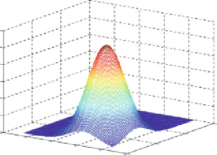
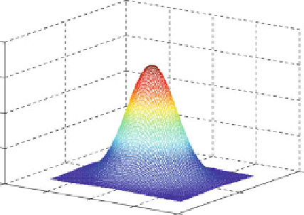
Fig. 3.36
Joint PDFs (
a
)
X
1
¼ N
(0, 1);
X
2
¼ N
(0, 1) (
b
)
X
1
¼ N
(4, 4);
X
2
¼ N
(3, 9)
Exercise M.3.7
(MATLAB file
exercise_M_3_7.m
) Plot the joint density for the
variables
Y
1
and
Y
2
from Example 3.4.1:
8
<
:
y
1
2
s
2
y
1
2
ps
2
e
f
Y
1
Y
2
ðy
1
; y
2
Þ¼
y
1
0
0
y
2
2
p;
:
(3.335)
for
;
0
otherwise
:
Solution
The joint density is shown in Fig.
3.37
.


Search WWH ::

Custom Search