Geoscience Reference
In-Depth Information
Fig. 2.14
An example of
proportional effect from a
West-African gold deposit.
Cell averages and standard
deviations are both in g/t
Example of Proportional Effect
Au
4.0
3.6
3.2
2.8
2.4
2.0
1.6
1.2
0.8
0.4
0.0
0.0
0.2
0.4
0.6
0.8
1.0
1.2
1.4
1.6
1.8
2.0
Cell Average
The most common statistics analyzed are the mean and stan-
dard deviations of the data within the windows.
A plot of the mean versus standard deviation calculated
from moving windows of data can be used to assess changes
in local variability, see Fig.
2.14
for an example. General-
ly, positively skewed distributions will show that windows
with higher local mean usually exhibits higher local stan-
dard deviation. This is the proportional effect described by
various authors, for example David (
1977
) and also Journel
and Huijbregts (
1978
). The proportional effect is due to a
skewed histogram, but it may also indicate spatial trends or
a lack of spatial homogeneity. Proportional effect graphs are
sometimes used to help determine homogeneous statistical
populations within the deposit (see Chap. 4).
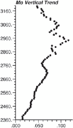
Fig. 2.15
Example of a
molybdenum vertical trend
2.3.4
Trend Modeling
Trend modeling is applied when a trend has been detected
and is assumed to be well understood. While some geosta-
tistical estimation methods are quite robust with respect to
the presence of trends, such as Ordinary Kriging (Chap. 8;
Journel and Rossi
1989
), there are many others, most notably
simulation (Chap. 10) that are quite sensitive to trends.
The trend is modeled as a deterministic component plus
a residual component. The deterministic component is re-
moved and then the residual component is modeled either
through estimation or simulation techniques. Finally, the de-
terministic trend is added back. In such a model, the mean
of the residual and the correlation between the trend and the
residual should be close to 0.
The drill hole data is typically the source for trend de-
tection. In some cases where the geological environment is
well understood, trends can be expected and modeled with-
out the drill hole data, but this should only be attempted
when there is no other option. Large scale spatial features
can be detected during several stages of data analysis and
modeling. Sometimes a simple cross-plot of the data against
elevation may show a trend, as in the example of Fig.
2.15
.
In other cases, simple contour maps on cross-sections, lon-
gitudinal sections, or plan views are enough to identify and
model trends. Moving window averages can also provide
an indication of whether or not the local means and vari-
ances are stationary. If there are notable changes in the local