Geoscience Reference
In-Depth Information
ferent anisotropies for different grade ranges is entirely
appropriate, since they have been validated with geologic
knowledge, ascribing them to different mineralization
controls.
14.5.4
Conditional Simulation Model
The conditional simulation model was obtained on a
5 × 5 × 5 m grid, and the volume modeled is such that it re-
sults in a model with more than 40 million nodes. Although
not every simulated node is retained in the end, the model
was run for the complete grid, although including the restric-
tion that at least one real 5 m composite is in the neighbor-
hood of the node before the simulated value can be obtained.
After the simulated model is obtained, it is restricted to the
areas where the 0.1 % TCu mineralized envelope exists, as
mentioned above. In this exercise, and largely due to time
constraints, 10 grade realizations were run.
The model is based on a two-stage simulation. First, the
geologic model was simulated using SIS on the categorical
variables that define the lithology package (Volcanic Brec-
cias, Andesites, or Intrusives). The output from this stage
is a model representing the probability that each unit exists
at a given node. Due to logistics and time constraints, the
simulated lithology was used as prior probability distribution
to condition grade estimation (as opposed to use as a direct
conditioning of the grade simulation).
The purpose of this first stage is to inject into the model
the relationship between grade and lithology. For example,
a node with a high probability of being a Volcanic Breccia
is more likely to have better grades than one with a high
probability of being an Andesite. This relationship between
lithology and grade is input into the grade simulation as prior
distributions of possible Cu grades for each node simulated.
The local declustered statistics of the 5 m composites were
used to derive these prior probability models for each area
within the deposit. For example, for Lince, the 5 m compos-
ites tagged as volcanic breccias indicate that a node simulat-
ed as volcanic breccia has a 57 % probability of having less
than 0.2 % TCu in grade. For Andesites, the same probability
is 64 %, while for those simulated as Intrusives it is 71 %.
Also, there is a 10 % probability that the nodes simulated as
volcanic breccias have a grade greater than 3 % TCu, while
this percentage is 3.2 % and 2.8 % for Andesites and Intru-
sives, respectively. This information is compiled for each
threshold used, and used as soft information in the form of
prior probability distributions.
The second step necessary to obtain the final simulated
model is to use the prior grade distributions assigned to each
node, as well as the 5 m composites themselves to simulate a
Cu grade in each node. The SIS model used a search ellipsoid
with a nominal 25 m search radius, with anisotropic ranges
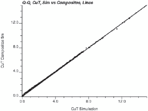
Fig. 14.51
Comparison of simulated values vs. 5 m composites and
blast holes, TCu, Lince
14.5.3
Indicator Variograms for TCu
and by Geologic Unit
The indicator method requires that an indicator variogram
model be obtained for each of the 11 thresholds defined
above. In addition, there should be one set of indicator mod-
els per GU considered, and per subzone or area in the depos-
it. So in total 33 indicator variogram models are required per
subzone of the deposit. In addition, three major zones were
defined for the purpose of variogram modeling (Lince, D4
and Hilary combined, and Estefanía), resulting in a total of
99 variogram models for the resource estimation and condi-
tional simulation model. Some observations regarding these
variogram models:
• The variogram models used for the resource estimation
are the same as those required for the conditional simu-
lation model. That is, this part of the work (as all other
required statistical work) is only done once, and used for
both the resource estimation and the conditional simula-
tion models.
• As expected, the variogram models for lower indicator
thresholds (waste or low grade) are more continuous than
the higher grade thresholds.
• As the indicator thresholds are increased, the overall
spatial correlation decreases, evidenced, for example, by
the increase of the nugget effect. This corresponds to the
intuitive notion that higher grade mineralization has less
spatial correlation than the more pervasive, lower grade
mineralization.
• There can be differences in anisotropy angles and ranges
for different grade ranges, as is the case for Lince-Este-
fanía. This is explained by different geologic controls
affecting parts of the grade distribution differently, for
example with a specific set of structures controlling the
higher grade mineralization. Therefore, modeling dif-