Geoscience Reference
In-Depth Information
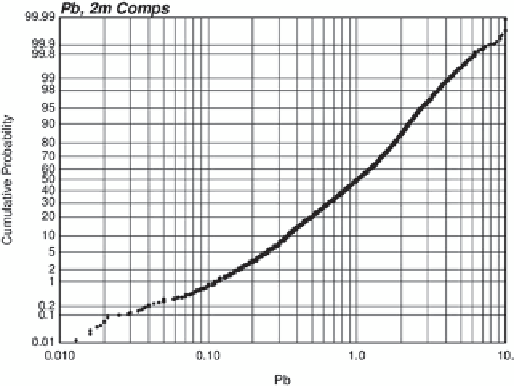
Fig. 2.3
An example of a probability plot. Data is lead concentration,
on 2 m composites, on a logarithmic scale
Fig. 2.2
Histogram of 2,993 data values. The common representa-
tion of the histogram has constant bin widths; the number of data in
each bin is labeled on this histogram
increases. There are techniques available for smoothing the
distribution, which not only removes such fluctuations, but
also allows increasing the class resolution and extending the
distributions beyond the sample minimum and maximum val-
ues. Smoothing is only a consideration when the original set
of data is small, and artifacts in the histogram have been ob-
served or are suspected. In practice, sufficient data are pooled
to permit reliable histogram determination from the available
data.
The graph of a CDF is also called a probability plot.
This is a plot of the cumulative probability (on the Y axis)
to be less than the data value (on the X axis). A cumula-
tive probability plot is useful because all of the data values
are shown on one plot. A common application of this plot
is to look at changes in slope and interpret them as dif-
ferent statistical populations. This interpretation should be
supported by the physics or geology of the variable being
observed. It is common on a probability plot to distort the
probability axis such that the CDF of normally distributed
data would fall on a straight line. The extreme probabilities
are exaggerated.
Probability plots can also be used to check distribution
models: (1) a straight line on arithmetic scale suggests a nor-
mal distribution, and (2) a straight line on logarithmic scale
suggests a lognormal distribution. The practical importance
of this depends on whether the predictive methods to be ap-
plied are parametric (Fig.
2.3
).
There are two common univariate distributions that are
discussed in greater detail: the normal or Gaussian and the
lognormal distributions. The normal distribution was first
introduced by de Moivre in an article in 1733 (reprinted in
the second edition of his
The Doctrine of Chances
, 1738) in
the context of approximating certain binomial distributions
for large
n
. His result was extended by Laplace in his topic
Fz dz
(
+−
)
Fz
()
fz
()
=
F z
'()
=
im
0
dz
→
dz
z
F z
()
=
−∞
f
()
z dz
The most basic statistical tool used in the analysis of data is
the histogram, see Fig.
2.2
. Three decisions must be made:
(1) arithmetic or logarithmic scaling—arithmetic is appro-
priate because grades average arithmetically, but logarithmic
scaling more clearly reveals features of highly skewed data
distributions; (2) the range of data values to show—the mini-
mum is often zero and the maximum is near the maximum
in the data; and (3) the number of bins to show on the histo-
gram, which depends on the number of data. The number of
bins must be reduced with sparse data and it can be increased
when there are more data. The important tradeoff is reduced
noise (less bins) while better showing features (more bins).
The mean or average value is sensitive to extreme values
(or outliers), while the median is sensitive to gaps or missing
data in the middle of a distribution. The distribution can be
located and characterized by selected quantiles. The spread
is measured by the variance or standard deviation. The coef-
ficient of variation (CV) is the standard deviation divided
by the mean; it is a standardized, unit-less measure of vari-
ability, and can be used to compare very different types of
distributions. When the CV is high, say greater than 2.5, the
distribution must be combining high and low values together
and most professionals would investigate whether the pool of
data could be subset based on some clear geological criteria.
Sample histograms tend to be erratic with few data. Saw-
tooth-like fluctuations are usually not representative of the
underlying population and they disappear as the sample size