Geoscience Reference
In-Depth Information
Location Map of Errors
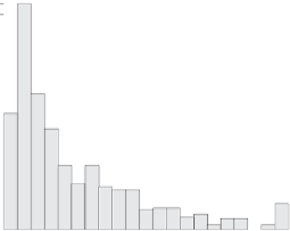
Au, Block Model
Number of Data55291
number trimmed 583178
mean 1.0604
std. dev. 1.0478
coef. of var0.9882
maximum5.5000
90th quantile 2.4500
upper quartile 1.5000
median 0.6600
lower quartile 0.3200
10th quantile 0.1900
minimum0.0000
0.200
5.0
4.0
0.150
3.0
2.0
1.00
0.100
.0
-1.00
0.050
-2.00
-3.00
-4.00
0.000
-5.00
0.00
1.00
2.00
3.00
4.00
Au (g/t)
Fig. 11.3
Histogram of estimated Au grades in g/t
Fig. 11.2
Location map of errors
Another check that can be performed, similar in concept,
is to assign geologic codes to blocks using the Nearest Neigh-
bor (NN) technique. The assumption is that the declustered
data (through NN) correctly represent the proportion of each
mineralization type and lithology within the deposit. Then it
is expected that the corresponding modeled volumes repre-
sent similar proportions for each minzone and lithologic unit.
There are a few caveats to this check. First, the assump-
tion is that the mapped and logged meters in the drill hole
database are representative. Spatial clustering or spatially
non-representative data is one possible source of error.
Additional possible discrepancies occurs if changes to the
originally mapped drill hole information are made as inter-
pretation progresses, and they are not incorporated into an
updated database. Sometimes the decisions are made at the
time of interpreting the units, and do not prompt a full-scale
re-logging or any changes in the database.
Also, the interpreted volumes may not be representative be-
cause some of the units are “border” units in the model. Thus,
they may be extended beyond what would be reasonable for
other units, as is the case with wall or host rock in Lithology
models. The check is applicable for the units that are well de-
limited within the model and enclosed by the outlying units.
parameters it is possible to better control the estimated
grades, including smoothing, contact grade profile reproduc-
tion, and global unbiasedness.
11.4.1
Geological Model Validation
The validation of the geologic model should be both statis-
tical and graphical. A discussion on graphical validation is
presented later in this chapter.
The geologic model is key in determining the tonnages
above cutoff of the resource model. This is because the
estimation domains generally define high, medium, low
grade, and barren zones. Those volumes with grades mostly
higher than the economic cutoff will be sent to the process-
ing plant. If the volumes of these zones have been over or
under-estimated, that error will directly translate into errors
in the corresponding tonnages above cutoff. In those circum-
stances, there is very little that geostatistics can do to correct
the volumetric bias.
The most common numerical check is by looking at the
proportions of each geologic unit in the database compared
to the proportions (volumes) of the modeled three-dimen-
sional solids. This is normally done by back-tagging the
composites used for resource estimation with the codes from
the modeled geologic units. Then, the statistics of each mod-
eled units can be compared to the original, logged intervals
that were used to create the model. Some discrepancies are
acceptable, as there may be some units too small or too com-
plicated to model, and some intercepts in the drill hole data-
base that are too narrow to be considered. A possible target is
to have a better than 90 % coincidence for each geologic unit
between the logged intervals and the back-tagged compos-
ites, but this percentage will vary depending on how com-
plex the geology is.
11.4.2
Statistical Validation
The basic statistical analysis compares means and variances
of the data and the model, including the spatial correlation
models in the case of simulations. In all cases, the drill hole
data used in these checks should be the same as the data used
to estimate the model, generally composites. This should be
done per estimation domain used to condition the estima-
tion or the simulation and using representative (declustered)
drill hole statistics for each domain. Figure
11.3
shows an
example of histogram of estimated Au values.