Geoscience Reference
In-Depth Information
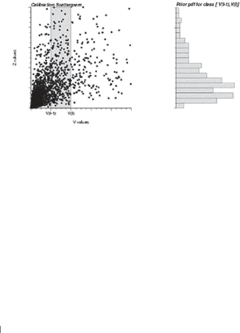
Fig. 10.15
Inference of the
soft prior probabilities from a
calibration scattergram. The prior
z probability pdf at a location
u′
α
where the secondary variable is
v(
u′
α
) in (v
l−1
, v
l
] is identified to
the calibration conditional pdf,
shown in the right of the figure
soft y indicator spatial distribution is likely different from
that of the hard i indicator data:
Consider a calibration data set {y(
u
α
; z), i(
u
α
; z), α = 1,…,n}
where the soft probabilities y(
u
α
; z) valued in [0,1] are com-
pared to the actual hard values i(
u
α
; z) valued 0 or 1. m
(1)
(z)
is the mean of the y values corresponding to i = 1; the best
situation is when m
(1)
(z) = 1, that is, when all y values exactly
predict the outcome i = 1. Similarly, m
(0)
(z) is the mean of the
y values corresponding to i = 0, best being when m
(0)
(z) = 0.
The parameter B(z) measures how well the soft y data
separate the two actual cases i = 1 and i = 0. The best case is
when B(z) = ± 1, and the worst case is when B(z) = 0; that is,
m
(1)
(z) = m
(0)
(z).
The case B(z) = − 1 corresponds to soft data predictably
wrong and is best handled by correcting the wrong probabili-
ties y(
u
α
; z) into 1 − y(
u
α
; z).
When B(z) = 1, the soft prior probability data y(
u
α
; z) are
treated as hard indicator data and are not updated. Converse-
ly, when B(z) = 0, the soft data y(
u
α
; z) are ignored; i.e., their
weights become zero.
Since the Y covariance model generally presents a
strong nugget effect, the Markov model implies that the
y data have little redundancy with one another. The un-
desired effect of this is that too much weight is given to
clustered, mutually redundant y data. In practice, only the
closest y datum is retained, which leads to using the col-
located correlation, i.e., the soft autocovariance at distance
0, C
Y
(h =
0
; z).
C zC
(;)
h
≠
(;)
h
zC z
≠
(;)
h
Y
IY
I
Then the indicator cokriging amounts to a full updating of all
prior cdf's that are not already hard.
At the location of a constraint interval j(
u
α
; z), indicator
kriging or cokriging amounts to in-filling the interval (a
α
, b
α
]
with spatially interpolated ccdf values. Thus if simulation
is performed at that location, a z attribute value would be
drawn necessarily from within the interval.
10.6.2
Markov-Bayes Model
With enough data one could infer directly and model the
matrix of covariance functions (one for each cutoff z):
[C
Y
(
h
; z) ≠ C
IY
(
h
; z) ≠ C
I
(
h
; z)]. An alternative to this te-
dious exercise is provided by the Markov-Bayes model,
whereby:
C
(;)
h
z
=
BzC
() (;),
h
z
∀
h
IY
I
2
C
(;)
h
z
=
B zC
() (;),
h
z
∀>
h
0
Y
I
=
Bz C
( )
( ;
h
z h
),
=
0
I
The coefficients B(z) are obtained from calibration of the
soft y data to the hard z data:
10.6.3
Soft Data Calibration
Consider the case of a primary continuous variable z(
u
) in-
formed by a related secondary variable v(
u
). The series of
hard indicator data valued 0 or 1, i(
u
α
; z
k
), k = 1,…,K, are
derived from each hard datum value z(
u
α
).
The soft indicator data, y(
u
α
,z
k
) in [0,1], k = 1,…,K, cor-
responding to the secondary variable value v(
u
α
), can be
(1)
( 0 )
Bz
()
=
m
()
z
−
m
() [1, 1]
z
∈− +
with:
m
(1)
()
z
=
EY
{(;) (;) 1}
u
z I
u
z
=
m
(0)
()
z
=
EY
{(;) (;) 0}
u
z I
u
z
=