Geoscience Reference
In-Depth Information
It generally takes only a few minutes on a capable computer,
and the coding is straightforward.
Other characteristics of the sequential annealing solution
is that it is straightforward to add components to objective
function; it often requires some trial-and-error to get the an-
nealing schedule right; but in the end, provides a solution to
an otherwise intractable problem.
The extension to geostatistical mining problems is
straightforward. First, an objective function must be formu-
lated which may include with many different components.
For example, local drill hole data with geologic information
and assays; variogram or other two-point spatial correlation
measures; multiple-point spatial connectivity, if available;
vertical and areal trends; correlation (collocated or spatial)
with secondary data; and historical data.
The objective function generally takes the form of a
weighted sum of multiple components. The basic approach
is the same:
1. Establish an initial guess;
2. Calculate the initial objective function;
3. Propose a change;
4. Update the objective function;
5. Decide whether to keep the change or not; this is the SA
decision rule;
6. Go back and propose a new change;
7. Stop when objective function is low enough. Generally,
this means that the original data is matched within accept-
able tolerances.
Simulated annealing provides a flexible optimization proce-
dure that has multiple applications and has not been fully
exploited within the mining industry. Partly this may be be-
cause the parameters need to be set up carefully to avoid
artifacts, such as the points where conditioning data exist,
and edge effects.
The annealing schedule may be difficult to establish, and
it generally requires some experience with the method to
avoid either lowering the temperature too slowly, with slow
Fig. 10.8
The traveling salesman needs to visit 100 cities within a
1,200 by 1,200 miles area
4. The annealing schedule is defined by choosing a starting
value of T larger than the largest change in energy ΔE
normally encountered. The procedure is complete when
nothing is happening, i.e., there is no improvement on the
Objective Function value (Fig.
10.8
).
Consider a N = 100 city problem within a 1,200 by
1,200 miles area:
Initially, choose randomly multiple configurations
(Fig.
10.9
) to assess what the non-optimal results would be.
A histogram of the total distance traveled of those multiple
configurations, 1,000 random paths in this case, is shown in
Fig.
10.10
.
The problem is solved with a near-optimal solution
(Fig.
10.11
) that results in 8,136 miles total distance traveled.
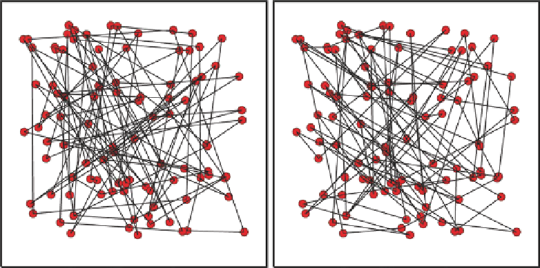
Fig. 10.9
Two initial
configurations chosen randomly