Geoscience Reference
In-Depth Information
In building a conditional simulation model, many of the
conditions and requirements of linear and non-linear estima-
tions apply, most importantly regarding stationarity deci-
sions. Shifts in geologic settings require the separation of
the data into different populations. Detailed knowledge of
the behavior of extreme and outlier values in the sampled
population is required. Issues such as limiting the maximum
simulated grade should be carefully considered.
The simulation method itself should be decided based on
the type of deposit, the Random Function model chosen, the
quantity and quality of available samples, the possibility of
using “soft” or fuzzy information, and the desired output.
All these are subjective decisions. These and other imple-
mentation parameters, along with the chosen algorithm and
simulated domain, have a bearing on the output simulations
and the uncertainty model.
Conditional simulation methods can be grouped in simi-
lar manner as estimation methods were in Chaps. 8 and 9.
There are simulation methods for continuous and discrete,
or categorical, variables; there are Gaussian and indicator-
based approaches, such as Sequential Gaussian (Isaaks
1990
) and Sequential Indicator (Alabert
1987a
). The latter is
more complicated, based on multiple indicator kriging tech-
niques, and requires definition of several indicator cutoffs.
The former is simpler and quicker, although more restrictive
in its basic assumptions. As with any estimation exercise,
variogram models are necessary.
There are other types of simulations, including object-
based simulation methods, and sequential annealing, a par-
ticular case of optimization. Also, there are several types of
multivariate simulations.
A conditional simulation model results in a set of
grades or realizations for each node. These realizations, all
equiprobable by construction, describe the model of uncer-
tainty for each block, i.e., provide the cumulative conditional
distribution function (ccdf) for that node. Preferably, a large
number of simulations are needed to describe the ccdf better.
However, a smaller number is generally used due to prac-
tical limitations. It has been these authors' experience that
between 20 and 50 simulations are generally sufficient to
characterize the range of possible values for the simulated
values
Uncertainty is not a property of the physical attribute
being modeled, but rather of the Random Function (RF)
model developed. The RF model includes the stationarity de-
cisions made; the simulation algorithms chosen; and the im-
plementation parameters used. Therefore, (a) the uncertainty
model that can be derived from conditional simulations is
subjective and only relevant to the underlying RF model; and
(b) applications or risk assessments that can be derived from
that uncertainty model are only useful and “realistic” if they
are relevant to the problem of interest.
A common example is the assessment of uncertainty of
a block model, used to define resources and reserves of a
Interpolation
Simulation
Equi-probable images with
same spatial variability as
reality
Smooth Version of
reality
Bad for modelling
extreme values
Good for modelling
extreme values
Fig. 10.1
Comparison of estimated and simulated models
deposit. The conditional simulation should be constructed
using the same underlying RF model used in the construc-
tion of the block model, if it is to describe resource uncer-
tainty. Likewise, the same geologic model and estimation
domains used to constrain the block model have to be used to
constrain the simulation model. Otherwise, the uncertainty
model will not fully relate to the resource model.
10.2
Continuous Variables: Gaussian-Based
Simulation
Gaussian simulations are most common in mining. Among
these, sequential Gaussian simulation (SGS) is the most fre-
quently used method, although there are several others that
are been used as well.
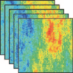
Gaussian methods are maximum entropy methods, in the
sense that for a specific covariance model, they provide the
most “disorganized” spatial arrangement possible. While
the covariance model controls the degree of mixing of high
and lows, there are some highly structured spatial distribu-
tions that may be more difficult to reproduce with a Gaussian
simulation (Fig.
10.2
). This results in a model that poten-
tially understates the continuity of the distribution's extreme
values. In practice, however, this effect can be controlled
through the definition of stationary geologic domains and
to some extent the covariance model. Gaussian simulations
are most popular because of their convenient properties and
easier implementation; but also because they result, for most
cases, in reasonable representations of spatial distributions.
The Turning Bands (TB) method was the first simula-
tion algorithm developed (Matheron
1973
; Journel
1974
), as
the simulation of a general trend plus a random error. It was
the only method available for several years, although never
applied in industry on a large scale. New methods, including