Geoscience Reference
In-Depth Information
9.9.2
Part Two: MG Kriging for Uncertainty
more relevant aspects. Subjective expressions of uncertainty,
assumptions and limitations, and recommendations for im-
provements should be included.
In addition, good practice requires a more detailed justi-
fication of the model. The main differentiation includes the
use of calibrations, and comparisons with alternative and
prior models. A comparison with past production should be
done, if available, and the model should be fully diluted. As
before, significant emphasis in describing uncertainty and
potential risk areas of the model should be discussed in de-
tail, and a risk mitigation plan should be suggested.
Best practice consists of using alternate models to check
the results of the intended final ore resource model. All rel-
evant production and calibration data should be used to indi-
cate whether the model is performing as expected, possibly
including simulation models to calibrate the recoverable re-
source model. The model should quantitatively describe the
amount of the different types of dilution included. All other
tasks related to checking and validation, model presenta-
tion, reporting, and visualization should also be completed.
Again, all risk issues should be dealt with in detail, and if
possible, quantified, which requires complementing the esti-
mation process with specific simulation studies.
The objective of this exercise is to become familiar with how
kriging can be used to get uncertainty without resorting to
simulation.
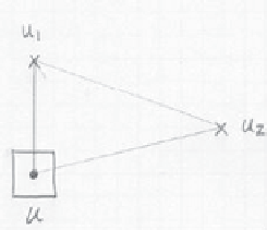
Copper grades in a particular domain were found to fit an
exponential distribution with a mean
m
of 1 %. Consider a
particular location
u
informed by two nearby samples at lo-
cations
u1
and
u2
such that |
u
-
u1
| = 20 m, |
u
-
u2
| = 37 m, and
|
u1
-
u2
| = 38 m. We are interested in the uncertainty in the cop-
per grade at the location
u
and in the uncertainty in the copper
grade of a 10 m cubed block centered at
u
. The copper grade
at
u1
is 2.5 % and the grade at
u2
is the mean value of 1 %.
Question 1:
Provide a detailed description of how you
would go about characterizing the uncertainty
about the unsampled value
z
(
u
) and calculat-
ing a best estimate and 90 % probability inter-
val. You are to adopt a multivariate Gaussian
model. State all the steps and approximations,
comment extensively, and use igures/sketches
where appropriate.
The multivariate distribution of the stationary copper grade
random function is assumed multinormal after appropriate
normal score transform. Variogram analysis was performed
on the standard normal transform of the copper grades. This
resulted in an isotropic spherical model with a nugget effect
of 10 % and a range of 100 m.
Question 2:
Write the equations for the transform to and
from Gaussian units. In general, the relation-
ship must be it, but it is possible to write equa-
tions in this case. Transform the data values to
Gaussian units. You can do this question on a
piece of paper with the help of a calculator.
Question 3:
Establish the parameters of the analytical con-
ditional distribution in Gaussian space. This
requires the solution of two equations with
two unknowns. Once again, this can be done
on paper with the help of a calculator.
Question 4:
Back transform 99 evenly spaced percentiles
to establish the conditional distribution in the
units of copper grade. You will probably want
to use Excel or a short program for this ques-
tion. Calculate the mean grade and the 90 %
probability interval.
9.9
Exercises
The objective of this exercise is to review indicator kriging
(IK) and multivariate Gaussian kriging (MG) for uncertainty
assessment. Some specific (geo)statistical software may be
required. The functionality may be available in different
public domain or commercial software. Please acquire the
required software before beginning the exercise. The data
files are available for download from the author's website—
a search engine will reveal the location.
9.9.1
Part One: Indicator Kriging
Question 1:
Consider the indicator variograms from Part 5
of Chap 6 using the
largedata.dat
data
ile. Setup indicator kriging to estimate with
the nine deciles as threshold values. You may
want to choose a smaller area near the centre
of the dataset. Run indicator kriging and create
a map at the median threshold for checking.
Question 2:
Post process the indicator kriging results to
calculate the local average (etype estimate) and
the local conditional variance. Map the results.
The local average should look like a kriged
map. The conditional variance should account
for the proportional effect, that is, higher grade
areas should have higher conditional variance
when the drillhole spacing is uniform.