Geoscience Reference
In-Depth Information
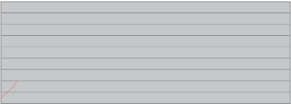
([WUDSRODWLQJ7UHQGV
(DVWLQJ
'DWDYDOXHV
&RQVWDQWWUHQG
/LQHDUWUHQG
([WUDSRODWHG&RQVWDQW
([WUDSRODWHG/LQHDU
Fig. 8.4
Sketch illustrating the differences between linear and constant trend extrapolations. Differences are quickly amplified for locations away
from actual data
trend if additional data allow focusing on the smaller-scale
variability. In the absence of physical interpretations, the
trend is usually modeled as a low-order (≤ 2) polynomial of
the coordinates
u
, e.g., with
u
=
(
x, y
):
• a linear trend in 1D: m(
u
) = a
0
+ a
1
x
• a linear trend in 2D limited to the 45° direction:
m(
u
) = a
0
+ a
1
(x + y)
• a quadratic trend in 2D: m(
u
) = a
0
+ a
1
x + a
2
y + a
3
x
2
+ a
4
y
2
+ a
5
x y
By convention,
f
0
(
u
)
= 1
, for all
u
. Hence the case
K = 0
cor-
responds to ordinary kriging with a constant but unknown
mean:
m
(
u
)
= a
0
.
Trend models using higher-order polynomials (n > 2)
or arbitrary non-monotonic functions of the coordinates
u
are better replaced by a random function component with a
large-range variogram.
When only
z
data are available, the residual covariance
C
R
(
h
) is inferred from linear combinations of
z
data that fil-
ter the trend
m
(
u
), as proposed by Delfiner (
1976
). For ex-
ample, differences of order 1 such as [
z
(
u
+
h
)
−
z
(
u
)] would
filter any trend of order zero
m
(
u
)
= a
0
; differences of order
2 such as [
z
(
u
+ 2
h
) −
2 z
(
u
+
h
)
+ z
(
u
)] would filter any trend
of order 1 such as
m
(
u
)
= a
0
+ a
1
u
.
However, in most practical situations it is possible to lo-
cate subareas or directions along which the trend can be ig-
nored, in which case Z(
u
) ≈ R(
u
), and the residual covariance
can be directly inferred from the local
z
data.
When the trend functions
f
k
(
u
) are not based on physical
considerations, as is often the case in practice, and in inter-
polation conditions, it can be shown that the choice of the
specific functions
f
k
(
u
) does not change the estimated values
z
KT
*
(
u
) or
m
KT
*
(
u
). When working with moving neighbor-
hoods the important aspect is the residual covariance
C
R
(
h
),
not the choice of the trend model.
The traditional notation for the trend does not reflect the
general practice of kriging with moving data neighborhoods.
Because the data used for estimation change from one loca-
tion
u
to another, the resulting implicit estimates of the pa-
rameters
a
1
's are different. Hence the following notation for
the trend is more appropriate:
K
=
u uu
m
()
af
() ()
k
k
k
=
0
The trend model, however, is important in extrapolation
conditions, i.e., when the data locations
u
α
do not surround
within the covariance range the location
u
being estimated.
Extrapolating a constant yields significantly different results
for either
z
KT
*
(
u
) or
m
KT
*
(
u
) than extrapolating either a line
or a parabola (non-constant trend), see Fig.
8.4
. However,
estimates based on extrapolation in mineral resource es-
timates are generally not acceptable per current Reporting
Standards (Chap 12). At most, a limited portion of resources
estimated in extrapolation conditions would be inferred,
which are deemed unreliable and not adequately known to
use in engineering studies and economic evaluations.
The practitioner is warned against overzealous modeling
of the trend and the unnecessary usage of universal kriging
(KT) or intrinsic random functions of order k (IRF-k, Math-
eron
1973
). In most interpolation situations the simpler and
well-proven OK algorithm within moving search neighbor-
hoods will suffice (Journel and Rossi
1989
). In extrapolation
situations, almost by definition, the sample
z
data alone can-
not justify the trend model chosen (Deutsch
2002
).