Geoscience Reference
In-Depth Information
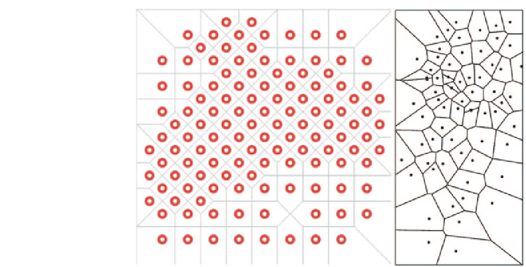
Fig. 8.3
Two schematic ex-
amples of the polygons of influ-
ence method; no distance units
are given
it is known that the errors are larger than for other meth-
ods. For many deposits with positively skewed distributions,
large errors in individual blocks lead to a tendency to over-
estimate the average grade and underestimate tonnage of the
resources above cutoff. The NN method is mostly used as a
checking tool (Chap. 11).
The second application is to decluster grades, assuming
that the block grade distribution is a fair representation of the
declustered drill hole data. While it is in concept equivalent
to a polygonal declustering technique, it is much easier to im-
plement, since most geologic and mining software packages
incorporate the algorithm. It can also be implemented as an
Inverse Distance method with specific parameters, see below.
The calculation of the weights
w
i
is based on inverse of
the distance between the composite and the point being esti-
mated. This is written as:
1
w
i
=
d
i
c
+
where
d
i
is the distance between the composite and the point
being estimated, ω is the exponent and c is a constant to
avoid over weighting very close data. The weights are stan-
dardized to sum to 1 to ensure a globally unbiased estimate.
Two generalizations are possible. One is to modify the ex-
ponent in Eq. 3.10. The most common exponents used are
ω = 2
(Inverse Distance Squared, IDS,) and
ω = 3
(Inverse
Distance Cubed, IDC,). IDS is used with smoothly varying
attributes, such as topographic surfaces, thickness of geo-
logic units including coal beds, some stratabound deposits,
and interpolation of in-situ bulk density values. Larger expo-
nents, such as
ω = 3
(IDC), are used when large weights are
desired for the closest composites. This is applicable when
the variable being estimated is more erratic and the current
data spacing is large relative to the data that will ultimately
be available for decision making, as for example with open
pit gold grade distributions. The extreme case is to increase
the exponent so that only the closest composite receives
any weight at all, which is equivalent to a nearest neighbor
estimation.
The opposite extreme is when the exponent is 0, which
amounts to an equally weighted moving average, as described
in Chap. 2. Isaaks and Srivastava (
1989
, pp. 257-259) dem-
onstrate the impact of the exponent on the weights assigned
to each composite.
8.1.8
Inverse Distance Weighting
Inverse Distance methods are a family of weighted average
methods. They result in estimates that are smoothed versions
of the original data. Inverse distance methods are based on
calculating weights for the samples based on the distrance
from the samples to the point or block of interest. The linear
estimator is written as:
N
w
i
·
z
i
i
=
1
∗
=
z
N
w
i
i
=
1
where
w
i
are the weights assigned to each composite data and
z
i
is the corresponding composite value, for all composites
(
i = 1,…, N
) used in the estimation, and
z
*
is the estimated value.