Geoscience Reference
In-Depth Information
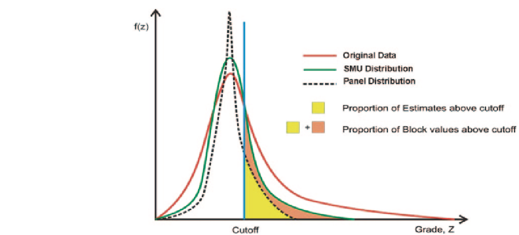
Fig. 7.7
Schematic showing vol-
ume-variance relations for origi-
nal data, SMU-sized distribution,
and a larger panel distribution
variance is the same expected squared difference as the vari-
ance defined before, except that it is related to specific sup-
port sizes for the data and the mean.
The dispersion variance can be expressed as a function of
average covariances or variograms, see Isaaks and Srivas-
tava (
1989
) or Journel and Huijbregts (
1978
):
value for all possible pairs within the block. The number of
discretization points used to estimate
D
2
(
v
,
V
) affects some-
what its final value. As a rule of thumb, it is generally ac-
cepted that a 5 × 5 × 5 grid of points within the SMU block is
sufficient to obtain a robust estimate of
D
2
(
v
,
V
)
.
Consider-
ing too many discretization points could lead to numerical
precision problems. One option is to obtain the dispersion
variance for several discretization grids. Figure
7.8
shows
the resulting dispersion variance for a given variogram
model and SMU size for several discretizing grids. Note how
the dispersion variance stabilizes after a reasonable number
of discretization points have been used.
The dispersion variance is a key parameter needed to
predict recoverable resources (recall Sect. 7.1). The volume-
variance correction is often characterized by a single param-
eter, known as the Variance Correction Factor (VCF). The
VCF (or more simply,
f
) is defined as the ratio of the SMU
block variance to the original sample variance:
D vV
2
(, )
=
C vv
(, )
−
CV V
( , )
(7.5)
where
C
(
v
,
v
) and
C
(
V
,
V
) are the average covariance val-
ues for the samples at smaller sample support
v
and the SMU
support respectively, as defined in Chap. 2. Note that these
are spatial averages, and therefore are location-independent.
The additive property of variances leads to the following
expression:
2
2
2
DvG
(, )
=
DvV
(, )
+
DVG
( , ),
∀⊂⊂
v V
G
(7.6)
where
v, V,
and
G
represent increasingly larger volumes.
Equation 7.6 states that the variance of samples within a
deposit can be found as the sum of the variance of samples
within blocks of a certain size plus the variance of those
blocks within the deposit. This relationship was found ex-
perimentally by D. Krige in the 1950's, and is thus often
called Krige's relation.
In Eq. 7.6 two terms are usually known: (1) the variance
of the data
D
2
(
v
,
G
)
=
DVG
2
( , )
DvG DvV
2
(, )
−
2
(, )
VCF
== =
f
D vG
2
(, )
D vG
2
(, )
D vV
D vG
(, )
2
2
=−
1
(7.7)
(, )
The factor
f
is a measure of how much the variance of a sam-
ple distribution will change, therefore giving an idea of the
importance of the volume-variance correction in the estima-
tion of recoverable resources. An
f
value close to one implies
that the variances of samples within the deposit (
D
2
(
v
,
G
))
and of SMU blocks (
D
2
(
v
,
G
)) within the deposit are fairly
similar. This is either because the SMUs are small (small
volume, highly selective mine), or the spatial distribution is
fairly continuous, that is, there is relatively little mixing of
σ
2
and (2) the variance within
blocks
D
2
(
v
,
V
), which can be estimated from the covari-
ance or variogram model (Eq. 7.1). The variance between
blocks (for example, the SMU variance within the Depos-
it,
D
2
(
V
,
G
) ) can be obtained.
The variance within blocks (
D
2
(
v
,
V
)) is obtained from
discretizing the SMU block
V
using
n
v
sample points, and
calculating the average covariance (
C
(
V
,
V
)) or variogram