Geoscience Reference
In-Depth Information
The interpretation of cross variograms is similar to that of
direct variograms; however, the sill of a cross variogram is
the collocated covariance C
k, k'
(0), which could be negative.
Thus, cross variograms may be both positive and negative;
they are the product of differences and not squared differ-
ences. The example shown below is for the case of negative-
ly correlated variables; thus when the spatial covariance C
k,
k'
(
h
) becomes zero, the cross variogram is at the collocated
covariance C
k, k'
(0), which is negative.
In presence of multiple variables, the set of
K
(
K
+ 1)/2
direct and cross variograms must be calculated, interpreted,
checked for geological reasonableness, then fitted by the
linear model of coregionalization (LMC). The LMC implic-
itly assumes that each variable is a linear combination of
common underlying random variables with zero mean. This
leads us to model all direct and cross variograms from the
same pool of
j = 0,…,nst
nested structures denoted with an
upper case Г
i
(
h
), where, by convention,
i
= 0 corresponds to
the nugget effect:
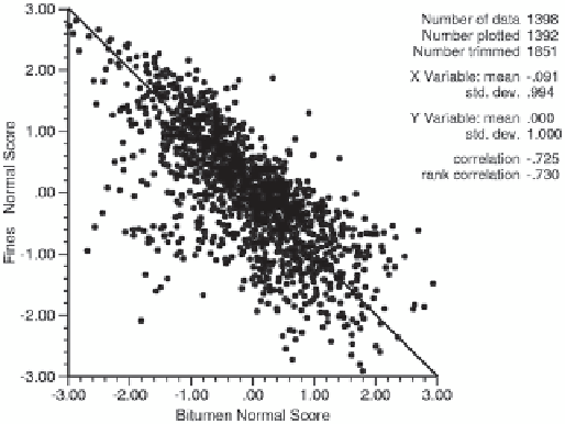
Fig. 6.11
Scatterplot of Gaussian bitumen and fines variables
and cross variograms together. A structure can exist in the di-
rect variogram and not exist in the cross variogram, but any
structure that occurs in the cross variogram must be in the di-
rect variograms. The variograms for normal score transforms
of % bitumen (Z) and % fines (Y) are shown:
nst
∑
i
i
γ
( )
h
=
b
i
Γ
( ),
h
kk
,
'
=
1,...,
K
kk
,'
kk
,'
i
=
0
The
b
coefficients are adjusted to fit the experimental
variograms just like the variance contribution parameters
are adjusted to fit the variograms of single variables. The
anisotropy and range parameters are also adjusted in the
specification of each constituent nested structure: Г
i
(
h
). It
will be necessary to use negative
b
coefficients for cross
variograms between variables that are negatively corre-
lated. The
b
coefficients can be adjusted as necessary to
achieve a good fit, but the resulting set of
K
(
K
+ 1)/2 di-
rect and cross variograms must be jointly positive definite.
This is achieved by ensuring that each of the
i
= 0,…,
nst
K
by
K
matrices of
b
coefficients is positive definite. There
are a number of software programs to ensure this including
spreadsheet plugins.
The following oil sands example illustrates a simple ap-
plication of a cross-variogram. Bitumen content and fines
content are two critical factors affecting recovery in the oil
sands. Evaluating their spatial variability is of some impor-
tance for process control in the extraction plant. Consider
the normal score transforms of the two variables, shown in
Fig.
6.11
:
A model of co-regionalization can be derived to account
for the cross correlation. Figure
6.12
shows the cross fines/
bitumen variogram.
The first step in fitting is to choose the pool of nested
structures Г
i,
i = 1,…,n
st
. Each nested structure is defined by
its type and ranges. It is chosen so that all of the deemed
significant features on the experimental variograms can be
modeled. The variograms may have different precision in
different directions, but it is important to look at all direct
γ
γ
γ
( )
h
=
0.3
+
0.3
⋅Γ
1
( )
h
+
0.25
⋅Γ
2
( )
h
+
0.15
⋅Γ
3
( )
h
Z
1
2
3
( )
h
= −
0.25
−
0.1
⋅Γ
( )
h
−
0.25
⋅Γ
( )
h
−
0.1
⋅Γ
( )
h
ZY
,
( )
h
=
0.4
+
0.2
⋅Γ
1
( )
h
+
0.25
⋅Γ
2
( )
h
+
0.15
⋅Γ
3
( )
h
Y
where
Г
1
(h) is spherical with range 200 m,
Г
2
(h) is spheri-
cal with range 1,000 m and
Г
3
(h) is spherical with range
5,000 m. This is a licit model of co-regionalization since
2
2
0.3 0.4
⋅ ≥−
( 0.25) , 0.3 0.2
⋅ ≥−
( 0.1) ,
2
2
0.25 0.25
⋅ ≥−
( 0.25) , and 0.15 0.15
⋅ ≥−
( 0.1)
The LMC can be applied to any number of variables, and
in all cases each matrix of
Г
coefficients should be positive
definite. For practical reasons, normally no more than 3 or
4 variables are considered simultaneously; otherwise, fewer
variables are considered or principal components of the orig-
inal variables are modeled instead.
6.5
Summary of Minimum, Good and Best
Practice
At a minimum, the variogram analysis performed should
include models for each variable within each estimation do-
main defined, an assessment of nugget effects and anisotro-
pies encountered in each case, and a detailed discussion on
their geological background. The documentation of the work
should be detailed, highlighting the approximations used, the