Geoscience Reference
In-Depth Information
study area may need to be subdivided if the direction of con-
tinuity changes systematically over the study area; but there
will be a trade-off between preserving local precision and
maintaining sufficient data for reliable calculations. Some
newer tools for locally varying anisotropy are becoming
available, but are not commonly used.
Variogram calculation is preceded by selection of the Z
variable to use in variogram calculation. The variable should
not be transformed for obtaining experimental variograms
for conventional kriging applications. The use of Gaussian
techniques requires a prior normal score transform of the
data and the variogram of those transformed data. Indicator
techniques require an indicator coding of the data prior to
variogram calculation.
Another aspect of choosing the correct variable is outlier
detection and removal. Extreme high and low data values can
have a large influence on the variogram value since each pair
is squared in the calculation. While erroneous data should be
removed, legitimate high values may also mask the spatial
structure of the majority of the data. The increased variability
of high values combined with preferential sampling in high
valued areas can lead to experimental variograms that are
noisy and difficult to interpret. Logarithmic or normal score
transformation mitigates the effect of outliers, but an appro-
priate back transform is being considered in later calculations.
The correct variable also depends on how trends are
going to be handled in subsequent model building. Some-
times, clear areal or vertical trends are removed prior to geo-
statistical modeling and then added to geostatistical models
of the residual (original value minus trend). If this two-step
modeling procedure is being considered, then the variogram
of the residual data is required. There is a risk, however, of
introducing artifact structures in the definition of the trend
and residual data.
The variogram is calculated for distance/direction lags
where there are a sufficient number of paired data. The var-
iogram is the average of squared differences from data pairs:
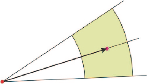
Fig. 6.3
Example tolerance for variogram calculation. The
bold arrow
between the two colored dots represents the vector of interest. Any vec-
tor from the right hand side dot to any location in the shaded area will
be accepted
times. This depends on the data configuration and the toler-
ance parameters.
Establishing the variogram tolerance parameters is trial
and error. If tolerances are too small, then the variogram will
be noisy. If tolerances are too large, then the spatial continu-
ity will be averaged out and imprecise. In general, lag and
angle tolerances should be set as small as possible to ensure
good definition of directional continuity while still obtaining
a stable variogram.
The maximum number of lags should be so that the maxi-
mum lag distance is less than one half of the domain size.
The variogram is only valid for a distance of one half of the
field size since for larger distances the variogram begins to
leave data out of the calculations. The lag tolerance is usu-
ally one half the lag separation distance. In cases of erratic
variograms or few data, the lag tolerance can be greater than
one half the lag separation to add additional pairs to the var-
iogram calculation and to smooth between lags.
The choice of directions for variogram calculation de-
pends on the anticipated anisotropy of the geological vari-
able, the number of samples available and the software used.
The geologic characteristics of the deposit can be understood
by looking at sections and plan views to define potential
directions of anisotropy. The orientation of the drill holes
should also be considered. If there are enough samples, mul-
tiple directions are reviewed before choosing a set of three
perpendicular directions. These three directions then become
the three main axes of the ellipsoid that represents the an-
isotropy.
An omnidirectional variogram considers all possible di-
rections simultaneously by opening the angle tolerance to
90°; they often yield the best-behaved variograms, but all
directional characteristics are lost. A down-the-hole vario-
gram will provide a good estimate of the nugget effect, as
well as the short scale continuity, since it is calculated from
adjacent data along the drill holes paths, without considering
their orientation.
N
∑
h
()
1
2 ( )
γ
h
[ (
z
u uh
)
−+
z
(
)]
2
(6.4)
i
i
N
()
h
i
=
1
It is rare to find data pairs exactly the same distance apart.
This requires that the
N
(
h
) pairs be assembled using reason-
able distance and direction tolerances (Fig.
6.3
). Variogram
calculation programs scan over all pairs and assemble the
ones that fall into approximate distance/direction
h
lags after
applying the specified tolerances. These tolerances define
sectors within which separation vectors are defined.
A simple 2-D example of this is shown in Fig.
6.4
. The
experimental variogram is the average squared difference
between the 16 pairs. Notice how some data are not used,
some are used once, some twice, and one data is used three