Geoscience Reference
In-Depth Information
ignored (not used) or reset to the top value defined, respec-
tively. Ignoring the outlier values altogether is not recom-
mended, since it tends to be overly conservative. More com-
monly, practitioners will reset all assays above the specified
cutoff to that value.
For some estimation and simulation methods, the treat-
ment of outlier values is accomplished within the method
itself. For example, if using multiple indicator kriging, the
impact of high values may be dealt through the definition
of a more conservative value for the upper class mean, see
Chap. 9.
For most cases, it is preferable to restrict the spatial influ-
ence of the outlier values at the time of estimation or simula-
tion. This is implemented in some software packages. The
assumption is that extreme values are valid and should be
used to estimate resources, but their spatial influence should
be limited. The high grade may be constrained to small-
size veinlets, or represent a nugget with little or no spatial
extension.
Capping the grades removes metal from the distribution
and limits the influence of the outliers. There may still be a
region of high estimates around the outliers, yet there may
be isolated high grade. The local estimates are checked on a
case-by-case basis.
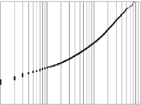
Au, Min. Prorphyry, Assays
99.99
99.
9
99.
8
9
99
95
90
80
6
70
50
3
40
20
10
5
2
0.
2
0.
1
0.01
0.010
0.10
1.0
10.
AU
Fig. 5.18
Probability plot, Au grade in a porphyry copper deposit
It is preferable to define a range of possible cutoff val-
ues for studying outliers. An example, taken from the Chang
Shan Hao Au deposit in Inner Mongolia, China, is shown in
Table
5.1
. The impact in terms of quantity of metal (QM) of
samples above a series of grade cutoffs is presented. Note
that, for example at the 4.0 g/t Au cutoff, just over 40 m of
samples, representing about 0.49 % of the total meterage in
the database, is responsible for over 5.7 % of the total quan-
tity of metal. Although this is not a very extreme case if
compared to other Au deposits, it indicates that outliers must
be considered to avoid overestimation when estimating the
resources for this deposit.
Statistical methods can also be used to determine the
impact and modeling of outlier grades. One such method,
proposed originally by Parker (
1991
), is based on assuming
specific distributions for the upper tail of the grade distribu-
tion including a log-normal distribution.
Another method, also proposed originally by Parker (per-
sonal communication), is to assume that, above a certain grade
threshold, the grade values are uncorrelated and independent
of each other. In this case, a Monte Carlo method is used,
whereby the high grade distribution is simulated. The amount
of metal that must be removed from the database is estimated
based on the simulated high grade distribution and for a speci-
fied condition. The condition is generally that the predicted
metal production on a yearly basis (for example) can be as-
sured with a given confidence level. This concept of analyzing
the problem from the perspective of mining risk is appealing,
but it has the caveat of the data independence related to the
Monte Carlo simulation, which is not always applicable. Also,
the distribution of outlier grades must be fairly homogeneous
for the metal to be accurately predicted by mining period.
To limit the influence of the outlier data, the most com-
mon procedure is to define a cutting or capping grade where-
by all samples above the specified grade cutoff are either
5.7
Density Determinations
In-situ density must be modeled at the time of resource esti-
mation. The predicted tonnage of the ore deposit is directly
dependent on the tonnage factor or density applied to the
modeled volumes.
A geologic model is used to predict the mineralized vol-
ume, and this volume in turn is multiplied by its in-situ den-
sity to obtain an estimated tonnage for the deposit. Any error
made in density determination and estimation is directly in-
corporated into tonnage estimates. A good discussion on this
issue can be found in Parrish (
1993
).
Several factors affect bulk density determinations such as
heterogeneity of the materials being sampled, the method of
determination, the practice of determining dry or wet densities,
rocks with voids in them (“vuggy” breccias, for example), the
material consolidation, relationships between ore grade and
densities, such as in massive sulfide deposits, and so on.
Immersion methods are commonly used to determine the
density of rock samples. The sample is weighed in air and
then in water. Density is then determined as:
†
W
‡
Density
=
ˆ
air
(5.2)
‰
Š
WW
−
‹
air
water
where
W
air
is the dry weight of the sample, and
W
water
is
the weight of the submerged sample. In practice, since it is