Information Technology Reference
In-Depth Information
7000
6000
5000
4000
3000
2000
1000
0
1
2
3
4
5
6
7
8
9
10
t
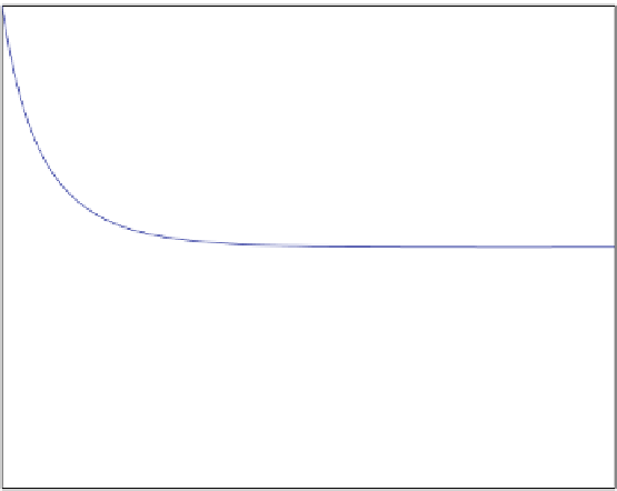
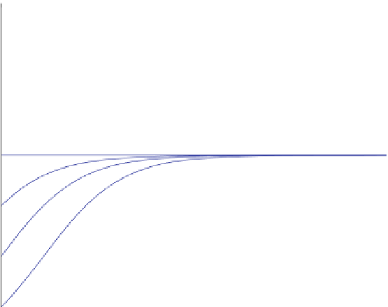
Fig. 2.1
Different solutions of (2.21) using different values of r
0
In Fig.
2.1
, we show seven different solutions of (2.21)usinga
D
1, R
D
4; 000,
and seven different initial values r
0
D
k
1; 000,fork
D
1;:::;7.
From Fig.
2.1
we note that whatever positive initial condition r
0
we give, the
solution ends up as r
D
R as time goes to infinity. This is also easy to see from the
analytical solution (2.21): Let t go to infinity; then the term e
at
goes to zero,
8
and
consequently r.t/ approaches R:
2.2
Numerical Solution
We have seen that it is possible to derive models of population growth using dif-
ferential equations. The models we derived are so simple that analytical arguments
are indeed sufficient to tell us all we ever want to know about the solutions. Unfor-
tunately, this is very rare in real-life applications. Analytical tools can solve very
few realistic models of nature. When analytical methods are inadequate, we have to
rely on numerical computations performed on computers. Now, do not let this lead
you to believe that finding analytical solutions of differential equations is a useless
8
Recall that a>0: