Information Technology Reference
In-Depth Information
8
6
4
2
0
−2
−4
−6
−8
0
0.1
0.2
0.3
0.4
0.5
0.6
0.7
0.8
0.9
1
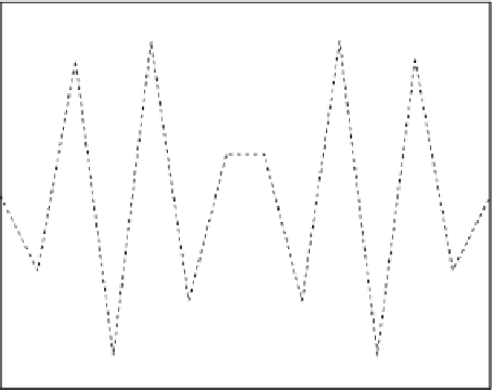
Fig. 7.20
Same problem as in Fig.
7.18
, but now the numerical solution corresponds to ˛
D
0:6760 > 0:5. The method fails to solve the problem under consideration
diffusion equation is only
conditionally stable
.Thismeansthatt cannot exceed a
critical value. This critical value corresponds to ˛
D
0:5, i.e., we must require that
t
1
2
x
2
:
(7.107)
This is the
stability criterion
of our numerical method.
7.4.6
A Discrete Algorithm Directly from Physics
The mathematical modeling of diffusion phenomena in this chapter starts with
physical principles, expressed as integral formulations, followed by the deriva-
tion of a differential equation, which is then discretized by the finite difference
method to arrive at a discrete model suitable for computer simulation. This section
outlines a different way of reasoning, where we start with the physical princi-
ples and go directly to a discrete computational model, without the intermediate
differential equation step. Many physicists and engineers prefer such an approach
to computerized problem solving.
We focus on the diffusive transport of a substance. Mass conservation in an
interval ˝ was expressed in Sect.
7.3.1
as
%q.a/t
%q.b/t
C
Z
b
a
%f t d x
D
Z
b
a
%c dx;
(7.108)