Information Technology Reference
In-Depth Information
1.2
1
0.8
0.6
0.4
0.2
0
0
0.1
0.2
0.3
0.4
0.5
0.6
0.7
0.8
0.9
1
ln
10
sin.t /
e
t
(
solid curve
) and a linear approximation
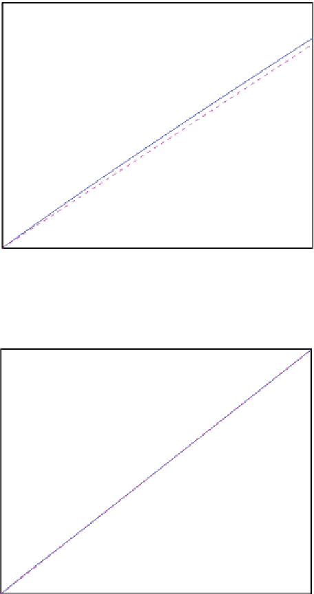
Fig. 5.16
The function y.t/
D
C
2
(
dashed line
) on the interval t
Œ0; 1
10
9
8
7
6
5
4
3
2
1
0
0
1
2
3
4
5
6
7
8
9
10
ln
10
sin.t /
e
t
(
solid curve
) and a linear approximation
Fig. 5.17
The function y.t/
D
C
(
dashed line
) on the interval t
2
Œ0; 10
But this is, of course, just pure luck and the example was constructed to obtain
exactly this effect. We obviously need a more systematic way of computing
approximations of functions. And that is the purpose of this section: to provide
methods for computing constant, linear and quadratic approximations of functions.