Information Technology Reference
In-Depth Information
1
0.9
0.8
0.7
0.6
0.5
0.4
0.3
0.2
0.1
0
0.1
0.2
0.3
0.4
0.5
0.6
α
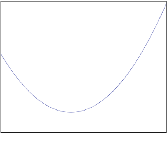
*=0.312
Fig. 5.6
A graph of F
D
F.˛/ given by (
5.2
)
and also
1
X
G
00
.˛/
D
12
.˛
y
i
/
2
:
(5.10)
i D1
Since G
00
.˛/ > 0,
2
we have a unique minimum and we compute this by solving
G
0
.˛
/
D
0:
(5.11)
Now, (
5.11
) is a third-order equation and such equations are in general difficult to
solve analytically. Instead, we use Newton's method. Consider Algorithm 4.2 on
page 108. By setting "
D
10
8
, ˛
0
D
0:312 and using G and G
0
as defined by (
5.8
)
and (
5.9
), respectively, we can run Newton's method to find
˛
0:345
in three iterations. In Fig.
5.7
, we have plotted G as function of ˛ for ˛
2
Œ0:1; 0:6
and we have marked the minimizing value ˛
0:345.
e
˛
,thenG
00
.˛/ > 0, but we do not have a minimum.
A more precise statement is as follows: If G is a smooth function with the property that G
00
.˛/ > 0
for all relevant ˛ and G
0
.˛
/
2
This is not completely accurate. If G.˛/
D
0,then˛
is a global minimum of G.
D