Hardware Reference
In-Depth Information
Step 1
: The algorithm invokes an
allocate
function which solves the actual MMKP
problem with the given constraints to produce a solution
γ
.
Step 2 and 3
: The invocation is performed iteratively until
γ
satisfies the given
constraints on the resources or all the application constraints have been relaxed
(
=
A
).
Steps 4, 5 and 6
: Whenever the solution is unfeasibl
e i
n terms of overall resources,
the deadline
τ
max
of the lowest priority application
α
is relaxed (Step 6) reducing
it to the minimum possible among a reduced set of resources
ρ
α
.
Step 7
:
allocate()
alg
o
rithm is invoked.
Step 8
: The selected
α
is then put into a
relaxed application set
.
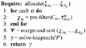
The
allocate
function (see Fig.
5.4
) actually solves the MMKP problem with a
light-weight algorithm as presented in [
38
].
Step 2
:
C
α
is pruned in order to have a single
φ
assignment for each
ρ
. This is
done by selecting only those configurations which meet
τ
max
but have the lowest
power consumption for a unique
ρ
. The resulting set of operating points is put
in
χ
α
and actually reduces the amount of data to be elaborated by the MMKP
solver considerably. Note that the pre-filtering Step 2 has a linear complexity with
respect to the cardinality of
C
α
due to the sorting performed in Fig.
5.2
, Step 11.
Step 4
:A
unified knapsack
vector
is created; this is a vector of
c
sorted by
prioritizing the
improvement
per single resource (
normalized user value
)
u
(
c
α
):
v
(
c
α
)
c
α
[
ρ
]
,
v
(
c
α
)
=
=
−
u
(
c
α
)
max
∀
c
∈
χ
α
c
[
π
]
c
α
[
π
]
(5.8)
In other words,
v
(
c
α
) is the improvement in terms of power consumption with
respect to the maximum power consuming operating point in
χ
α
.
u
(
c
α
)is
v
(
c
α
)
per unitary resource.
Step 5
: A greedy linear-scan algorithm [
38
] is invoked on
for identifying the final
set of operating points
γ
. Given the sorting performed previously, the algorithm
has a worst case complexity of
O
(
pN
log(
pN
)), where
N
is the average size of
the operating point set per application.
It can be shown that the total worst-case complexity of our RRM scheme is
O
(
pN
max
+
pN
log(
pN
)), where
p
is number of active applications,
N
is a set of all
active applications and
N
max
is maximum number of configurations. This reduction
in complexity is achieved due to the adequate filtering and sorting done before the
greedy algorithm solving the knapsack problem. Running such an algorithm on a
Fig. 5.4
Allocate function

Search WWH ::

Custom Search