Design Space Exploration Supporting Run-Time Resource Management - Multi-objective Design Space Exploration of Multiprocessor SoC Architectures - page 102

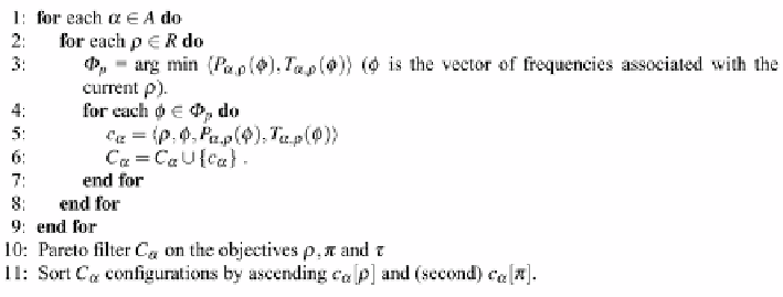
Fig. 5.2 Design-time methodology for identifying the initial C α , for each application α

and modeling techniques (see Chaps. 3 and 4) supported by DSE tool. The following
algorithm describes sequence of steps taken during our design-time methodology.
Algorithm in Fig. 5.2 shows the structure of adopted design-time methodology.
The algorithm mainly performs the minimization of the execution time and power
consumption for each application version (i.e., for each application α and each
available version of α which is parallelized over ρ resources).
Once all results are collected, these are sorted for obtaining a further speedup at
run-time. A more detailed step-by-step description follows:

￿ Steps 1, 2 and 3 : The algorithm loops over the set of available applications A (Step

1) and the set of resources R (Step 2) by solving a multi-objective minimization
problem with respect to both P α , ρ ( φ ) and T α , ρ ( φ ) (Step 3). In our case, P α , ρ ( φ )
and T α , ρ ( φ ) are, respectively, the average power consumption and the execution
time delay returned by the architectural simulator for a frequency configuration
vector φ . Note that the independent variable to be optimized is φ since ρ is set as
a constraint in the loop (Step 2).
Since the size of the design space increases rapidly with ρ , while for ρ ≤ 3a

full search exploration is performed, for ρ 4 the problem is solved by using

the NSGA-II multi-objective genetic algorithm [ 10 ]. The genetic algorithm is run
with a population size

≥

ρ for 50 generations. The set p contains all the
Pareto configurations associated with the solution of the problem.
￿ Steps 5 and 6 : The set p is used to construct the operating points and insert them
into the associated C α .
￿ Step 10 : It prunes C α from all the configurations that do not represent an efficient
trade-off in terms of resources, energy and execution time.
￿ Step 11 : It sorts the resulting C α to improve the performance of the run-time
algorithm while finding an operating point with a lower resource usage while
achieving τ max .
The proposed heuristic methodology is able to save a considerable number of simula-
tions. The exact amount of simulation time saving depends on the specific application
scenario as well as from the selected optimization algorithm used for solving the

| |×