Processing for compression - The MPEG - page 82

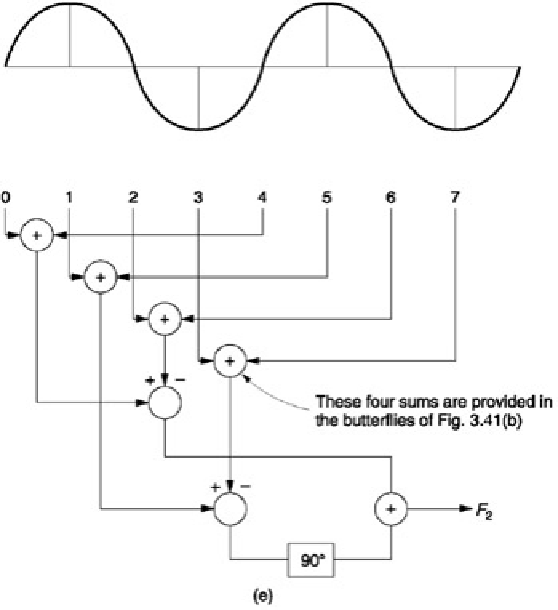
Figure 3.41: The basic element of an FFT is known as a butterfly as in (a) because of the shape of the signal paths
in a sum and difference system. The use of butterflies to compute the first two coefficients is shown in (b). An
actual example is given in (c) which should be compared with the result of (d) with a quadrature input. In (e) the
butterflies for the first two coefficients form the basis of the computation of the third coefficient.
Figure 3.41 (c) shows a numerical example. If a sine wave input is considered where zero degrees coincides with
the first sample, this will produce a zero sine coefficient and non-zero cosine coefficient. Figure 3.41 ( d) shows the
same input waveform shifted by 90°. Note how the coefficients change over.
Figure 3.41 (e) shows how the next frequency coefficient is computed. Note that exactly the same first-stage
butterfly outputs are used, reducing the computation needed.
A similar process may be followed to obtain the sine and cosine coefficients of the remaining frequencies. The full
FFT diagram for eight samples is shown in Figure 3.42 (a). The spectrum this calculates is shown in Figure 3.42 (b).
Note that only half of the coefficients are useful in a real band-limited system because the remaining coefficients
represent frequencies above one half of the sampling rate.