Processing for compression - The MPEG - page 77

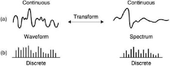
Figure 3.37: Continuous time signal (a) has continuous spectrum. Discrete time signal (b) has discrete spectrum.
Duality also holds for sampled systems. A sampling process is periodic in the time domain. This results in a
spectrum which is periodic in the frequency domain. If the time between the samples is reduced, the bandwidth of
the system rises. Figure 3.37 (a) shows that a continuous time signal has a continuous spectrum whereas at (b) the
frequency transform of a sampled signal is also discrete. In other words sampled signals can only be analysed into
a finite number of frequencies. The more accurate the frequency analysis has to be, the more samples are needed
in the block. Making the block longer reduces the ability to locate a transient in time. This is the Heisenberg
inequality which is the limiting case of duality, because when infinite accuracy is achieved in one domain, there is
no accuracy at all in the other.
3.12 The Fourier transform
Figure 3.35 showed that if the amplitude and phase of each frequency component is known, linearly adding the
resultant components in an inverse transform results in the original waveform. The ideal Fourier transform operates
over an infinite time. In practice the time span has to be constrained, resulting in a short-term Fourier transform
(STFT). In digital systems the waveform is expressed as a (finite) number of discrete samples. As a result the
Fourier transform analyses the signal into an equal number of discrete frequencies. This is known as a discrete
Fourier transform or DFT in which the number of frequency coefficients is equal to the number of input samples.
The fast Fourier transform is no more than an efficient way of computing the DFT. [ 14 ]
It will be evident from Figure 3.35 that the knowledge of the phase of the frequency component is vital, as changing
the phase of any component will seriously alter the reconstructed waveform. Thus the DFT must accurately analyse
the phase of the signal components.
There are a number of ways of expressing phase. Figure 3.38 shows a point which is rotating about a fixed axis at
constant speed. Looked at from the side, the point oscillates up and down at constant frequency. The waveform of
that motion is a sine wave, and that is what we would see if the rotating point were to translate along its axis whilst
we continued to look from the side.
One way of defining the phase of a waveform is to specify the angle through which the point has rotated at time
zero ( T = 0). If a second point is made to revolve at 90° to the first, it would produce a cosine wave when
translated. It is possible to produce a waveform having arbitrary phase by adding together the sine and cosine
wave in various proportions and polarities. For example, adding the sine and cosine waves in equal proportion
results in a waveform lagging the sine wave by 45°.