Audio compression - The MPEG - page 127

Figure 4.42: Transform duality suggests that predictability will also have a dual characteristic. A time predictor will
not anticipate the transient in (a), whereas the broad spectrum of signal (a), shown in (b), will be easy for a
predictor advancing down the frequency axis. In contrast, the stationary signal (c) is easy for a time predictor,
whereas in the spectrum of (c) shown at (d) the spectral spike will not be predicted.
Equally, a predictive coder working in the time domain produces an error spectrum which is related to the input
spectrum. The dual of this characteristic is that a predictive coder working in the frequency domain produces a
prediction eror which is related to the input time domain signal. This explains the use of the term temporal noise
shaping (TNS) used in the AAC documents. [ 28 ] When used during transients, the TNS module produces distortion
which is time-aligned with the input such that pre- echo is avoided. The use of TNS also allows the coder to use
longer blocks more of the time. This module is responsible for a significant amount of the increased performance of
AAC.
Figure 4.43 shows that the coefficients in the transform block are serialized by a commutator. This can run from the
lowest frequency to the highest or in reverse. The prediction method is a conventional forward predictor structure in
which the result of filtering a number of earlier coefficients (20 in main profile) is used to predict the current one.
The prediction is subtracted from the actual value to produce a prediction error or residual which is transmitted. At
the decoder, an identical predictor produces the same prediction from earlier coefficient values and the error in this
is cancelled by adding the residual.
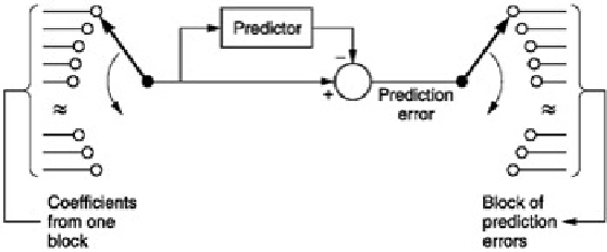
Figure 4.43: Predicting along the frequency axis is performed by running along the coefficients in a block and
attempting to predict the value of the current coefficient from the values of some earlier ones. The prediction error
is transmitted.
Following the intra-block prediction, an optional module known as the intensity/coupling stage is found. This is used
for very low bit rates where spatial information in stereo and surround formats is discarded to keep down the level
of distortion. Effectively over at least part of the spectrum a mono signal is transmitted along with amplitude codes
which allow the signal to be panned in the spatial domain at the decoder.
The next stage is the inter-block prediction module. Whereas the intra- block predictor is most useful on transients,
the inter-block predictor module explores the redundancy between successive blocks on stationary signals. [ 29 ] This
prediction only operates on coefficients below 16 kHz. For each DCT coefficient in a given block, the predictor uses
the quantized coefficients from the same locations in two previous blocks to estimate the present value. As before
the prediction is subtracted to produce a residual which is transmitted. Note that the use of quantized coefficients to
drive the predictor is necessary because this is what the decoder will have to do. The predictor is adaptive and
calculates its own coefficients from the signal history. The decoder uses the same algorithm so that the two
predictors always track. The predictors run all the time whether prediction is enabled or not in order to keep the
prediction coefficients adapted to the signal.
Audio coefficients are associated into sets known as scale factor bands for later companding. Within each scale
factor band inter-block prediction can be turned on or off depending on whether a coding gain results.
Protracted use of prediction makes the decoder prone to bit errors and drift and removes decoding entry points
from the bitstream. Consequently the prediction process is reset cyclically. The predictors are assembled into